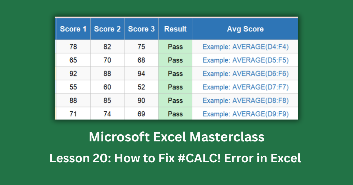
The #CALC! error is one of the newest entries in Excel’s error library. It arrived alongside dynamic array functions — FILTER, UNIQUE, SORT, SEQUENCE, MAKEARRAY, BYROW, and BYCOL — which began rolling out from Excel 2019 onward and are fully standard in Microsoft 365. If you’re on Excel 2016 or any older version, you won’t see this error at all because those functions don’t exist there. If you’re on a perpetual licence of Excel 2019 or 2021, you’ll see it only occasionally. Microsoft 365 subscribers encounter it most often as these newer functions spread through everyday spreadsheet work.
What does #CALC! mean? It means a formula completed its calculation but produced a result that Excel can’t use. The most common version: a FILTER formula that found zero matching rows. An empty array is technically a valid calculation output, but Excel can’t place “nothing” into cells — so it shows #CALC! instead. The formula isn’t wrong. The data just produced an empty result.
This post covers every cause of the #CALC! error with specific fixes for each, using a 25-student exam results dataset where FILTER, MAKEARRAY, and BYROW formulas each trigger the error in different ways.
Quick Takeaways:
- #CALC! is exclusive to Excel 2019, 2021, and Microsoft 365. Excel 2016 and earlier don’t have dynamic array functions and can’t produce this error.
- The most common cause is FILTER() returning zero matching rows. Add a third argument to FILTER as a fallback: =FILTER(range,condition,”No results”).
- MAKEARRAY, BYROW, and BYCOL require Microsoft 365 (2022+ builds). Excel 2019 and 2021 users will see #CALC! or #NAME? when these functions are used.
- LAMBDA is Microsoft 365 only. Any formula using LAMBDA on a perpetual Excel licence returns an error. Use nested IF or helper columns instead.
- IFERROR is the universal safety net: =IFERROR(FILTER(range,condition),”No data”) works across all versions that support FILTER.
What Causes the #CALC! Error in Excel
Unlike #VALUE! or #DIV/0! — which come from wrong data types or division by zero — #CALC! is specifically about dynamic array functions producing results that Excel can’t handle. There are three main categories.
Category 1: An Empty Array Result
The most frequent trigger. FILTER and UNIQUE are designed to return a list of matching results. When no data matches the condition, they return an empty array — and empty arrays can’t be displayed in cells.
In the student exam dataset, the formula =FILTER(B4:B28,D4:D28>95) looks for students who scored above 95. If no student reaches that threshold, FILTER has nothing to return. #CALC! appears immediately.
The same applies to UNIQUE on an empty range. If the source range has no values, UNIQUE can’t deduplicate anything. Result: #CALC!.
Category 2: A Function That Doesn’t Exist in the Current Excel Version
MAKEARRAY, BYROW, and BYCOL were added to Microsoft 365 in mid-2022. LAMBDA arrived in 2021. These are not available in Excel 2019, Excel 2021 (perpetual licence), or any older version. When someone on those versions opens a file using these functions, they see either #CALC! or #NAME? depending on their exact build.
This is a genuine organisational problem. A formula written on Microsoft 365 may behave completely differently when opened on an older version. Files shared across a team where not everyone is on the same Excel version will show errors for some users and work correctly for others.
Category 3: A Logically Impossible Condition
Less common but worth knowing. If a FILTER condition can never be true, the formula always returns an empty array and always shows #CALC!. In the exam dataset, =FILTER(A4:G28,D4:D28>100) asks for students who scored over 100 on a 100-point scale. No such student can exist. The formula will never return anything.
How to Fix #CALC! Error in Excel
Fix 1: Add the [if_empty] Argument to FILTER
FILTER has a third argument that most people don’t use. It’s designed precisely for the situation where the filter condition matches nothing.
=FILTER(B4:B28,D4:D28>85,”No students above 85″)
When at least one student scores above 85, the formula returns their names as normal. When no student qualifies, it returns the text “No students above 85” in a single cell instead of #CALC!. The formula stays in place and handles both outcomes gracefully.
For numeric columns, return 0: =FILTER(D4:D28,D4:D28>85,0). For situations where you want the cell to appear blank when empty: =FILTER(B4:B28,D4:D28>85,””) returns an empty string, which looks blank but doesn’t produce an error.
This is the cleanest fix and the one Microsoft’s FILTER function documentation recommends as the standard approach.
Fix 2: Wrap With IFERROR as a Universal Safety Net
=IFERROR(FILTER(B4:B28,D4:D28>85),”No results”) catches any error FILTER produces — not just #CALC!, but also #VALUE! or #SPILL! that could occur for other reasons.
IFERROR is available in Excel 2007 and all later versions, making it the most portable protection available. For teams where files move between different Excel versions, IFERROR is the safer wrapper because it doesn’t depend on the [if_empty] argument that requires a current Excel 365 build.
The trade-off: IFERROR hides all errors, including genuine formula mistakes. I find it’s better practice to add the [if_empty] argument directly when the issue is specifically a potentially empty FILTER result, and reserve IFERROR for cases where multiple error types might occur.
Fix 3: Replace MAKEARRAY, BYROW, and BYCOL With Version-Safe Alternatives
If your file is used by people on different Excel versions, these functions need safe fallbacks.
BYROW for row averages: =BYROW(D4:F28,LAMBDA(row,AVERAGE(row))) calculates the average of each row across three score columns. On older Excel, this fails. The version-safe equivalent: put =AVERAGE(D4:F4) in a single row and copy it down the column. It’s less elegant but it works in Excel 2007 and beyond.
For a single-formula approach that avoids BYROW on version-sensitive files, MMULT handles row-wise summation: =MMULT(D4:F28,{1;1;1})/3. MMULT has been in Excel since version 2000.
MAKEARRAY for generating grids: =MAKEARRAY(5,3,LAMBDA(r,c,r*c)) creates a multiplication table. On older Excel: use SEQUENCE combined with arithmetic to achieve the same result, or create the grid manually with a helper formula.
BYCOL for column operations: Replace with standard column formulas (SUM, AVERAGE, MAX applied per column) rather than the lambda-based BYCOL approach.
Fix 4: Replace LAMBDA-Based Functions for Cross-Version Files
LAMBDA arrived in Microsoft 365 in 2021. If a formula uses LAMBDA — directly or through MAP, SCAN, REDUCE, BYROW, or BYCOL — and it opens on Excel 2019 or a perpetual 2021 licence, #CALC! or #NAME? appears.
For grade assignment, a nested IF is the version-safe approach: =IF(H4>=90,”A”,IF(H4>=80,”B”,IF(H4>=70,”C”,IF(H4>=60,”D”,”F”))))
This works in Excel 2003 and beyond. For complex conditional logic that LAMBDA makes clean, helper columns with simple formulas are the pragmatic cross-version solution.
Fix 5: Check the Filter Condition for Logical Impossibilities
When FILTER always returns #CALC! regardless of the data, the condition itself is the problem. A score threshold above the maximum possible value will never match. A department filter looking for “Engineering” in a list that only contains “Finance”, “HR”, and “IT” will never match.
Before adding IFERROR or [if_empty] as a workaround, verify the condition makes sense. If it does make sense but just happens to match nothing right now, add [if_empty] as the correct fix. If the condition is logically impossible, fix the condition.
#CALC! vs #SPILL! vs #NAME?: Telling Them Apart
These three errors appear in similar contexts and are worth distinguishing clearly.
#CALC! means the calculation produced an unusable result — an empty array or a function with no valid output. The formula ran; the result was empty or impossible.
#SPILL! means the formula produced results but couldn’t write them anywhere because cells in the destination range are occupied. The formula produced output; there was nowhere to put it.
#NAME? means Excel didn’t recognise something in the formula — a misspelled function name, or a function that simply doesn’t exist in that Excel version. The formula never ran.
The confusion between #CALC! and #NAME? is most common with MAKEARRAY and BYROW: newer Microsoft 365 builds show #CALC!, while significantly older builds that don’t recognise the function name at all show #NAME?. Same root cause (wrong Excel version), different symptoms.
A One-Rule Prevention Habit
Add the [if_empty] argument to every FILTER formula you write, from the start. =FILTER(range,condition,”No results”) is a habit, not an afterthought. When you’re building the formula, you might be working with test data that always matches. The production environment often won’t. A FILTER formula without a fallback is a #CALC! error waiting to happen.
For teams mixing Microsoft 365 and older Excel versions, agree on a version baseline before using newer functions in shared files. The cost of rebuilding a workbook because half the team can’t open it correctly is much higher than using an older-but-compatible alternative from the start.
Open the practice file and compare the error sheet (with annotated FILTER, MAKEARRAY, and BYROW failures) against the fixed sheet to see each correction applied with clean data and proper fallbacks in place.