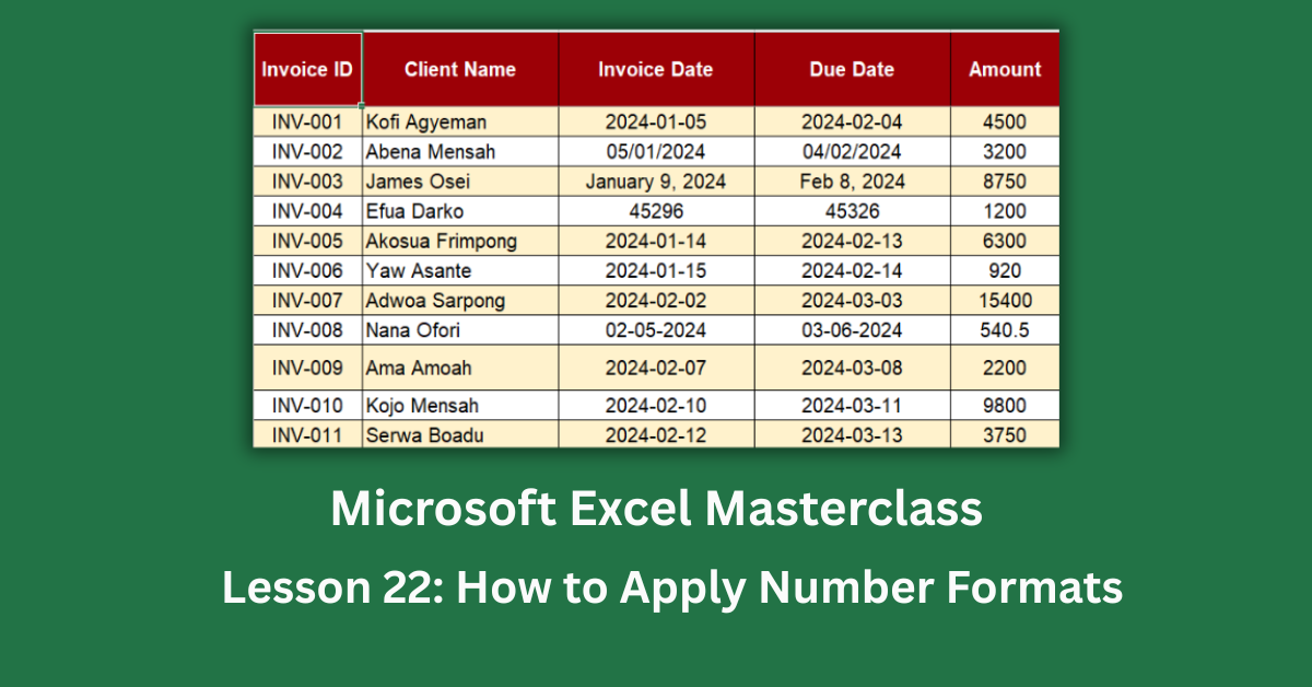
A spreadsheet full of raw numbers is like a report written in a foreign language. The data might be perfectly accurate, but if nothing is formatted, nobody knows what they’re looking at. Is that 15 a tax rate, a percentage, a unit count, or a dollar amount? Without applying the right number formats in Excel, you’re leaving your readers to guess.
This guide walks through exactly how to format currency, dates, and percentages in Excel, using a real 15-invoice dataset as the working example. Along the way, you’ll see the specific mistakes that quietly corrupt calculations and how to fix each one. These features are available in Excel 2016 and all later versions, including Excel 2019, Excel 2021, and Microsoft 365. Custom format codes and AVERAGEIF-based functions work in all of those versions too.
Quick Takeaways:
- Typing 15 when you mean 15% is one of the most common Excel errors. Apply % format to 0.15, not 15, or your totals will be 100x too large.
- Dates stored as serial numbers (like 45296) aren’t broken. They just need a date format applied via Ctrl+1.
- Numbers imported from other systems often arrive as text. A =VALUE() formula or Text to Columns fixes them in seconds.
- The $#,##0.00 format code gives you the standard professional currency display with dollar sign, comma separators, and two decimal places.
- DD-MMM-YYYY (e.g., 09-Jan-2024) is the safest date format because it removes all ambiguity across regions.
Why Number Formatting Matters More Than You Think
Here’s a scenario worth sitting with. The invoice dataset used throughout this post covers 15 clients, totalling $88,980.45 in invoices raised between January and March 2024. Of that, only $38,025.50 was collected. The outstanding balance sits at $50,954.95, and the collection rate is just 42.7%.
Those numbers tell a clear story. But in the raw, unformatted version of the same file, the total invoiced column just shows 4500, 3200, 8750 with no symbol, no comma, no unit. You genuinely can’t tell whether those are dollars, euros, units, or something else entirely. Three invoices show overdue balances averaging 25.9 days late. That urgency disappears completely when the numbers look like plain integers.
Formatting doesn’t change any of the underlying data. It changes whether anyone can act on it.
How to Apply Currency Formatting in Excel
The Basic Method
Select your currency cells, then press Ctrl+1 to open the Format Cells dialog. Go to the Number tab, choose Currency, set your symbol and decimal places, then click OK. For most invoicing or financial work, two decimal places is standard.
You can also use the Home > Number group and click the $ button for a one-click shortcut. That applies the default currency format for your system locale.
The Format Code That Professionals Use
I’ve found that the built-in currency options don’t always match what accountants and finance teams expect. For more control, use a custom format code. Press Ctrl+1, go to Custom, and enter:
$#,##0.00;($#,##0.00);”-“
This shows positive values as $5,175.00, negative values as ($2,530.00) in parentheses (standard financial convention), and zeros as a dash. In the dataset, the Balance column uses exactly this format. It makes overdue amounts like Ama Amoah’s $2,530.00 outstanding immediately recognizable as a problem.
The Mistake: Numbers Stored as Text
INV-002 (Abena Mensah) and INV-005 (Akosua Frimpong) both had their amounts stored as text, not numbers. You can spot this instantly: text-numbers are left-aligned in a cell, and you’ll often see a small green triangle in the top-left corner. The dangerous part? A SUM() formula on a text-number column returns zero. No warning, no error.
The fix is straightforward. Select the column, go to Data > Text to Columns, click Finish without changing any settings, and Excel converts the column back to real numbers. Alternatively, use =VALUE(A1) to convert a single cell.
How to Apply Date Formatting in Excel
Understanding How Excel Stores Dates
Excel stores every date as a serial number, where January 1, 1900 is 1. So January 11, 2024 is stored as 45296. That’s not a bug; it’s by design. It lets Excel calculate the number of days between two dates in a single formula.
The problem only occurs when a cell is formatted as General instead of Date. INV-004 in the dataset (Efua Darko) had exactly this issue. The Invoice Date showed as 45296 instead of 11-Jan-2024. Fix it by selecting the cell, pressing Ctrl+1, choosing Date, and picking your preferred display format. The underlying number stays 45296. Only the display changes.
Choosing a Date Format That Won’t Confuse Anyone
INV-008 (Nana Ofori) had the date entered as “02-05-2024”. Is that February 5th or May 2nd? Impossible to tell without knowing the user’s locale. This is a surprisingly common issue in shared spreadsheets used across countries.
The safest approach is DD-MMM-YYYY, which displays as 05-Feb-2024. Month as three-letter text removes all ambiguity. Apply it via Ctrl+1 > Date, or type the code directly in the Custom field.
For converting text dates like “January 9, 2024” to real date values, the =DATEVALUE() function does the job:
=DATEVALUE(“January 9, 2024”) returns 45300, which you then format as a date.
Microsoft’s full date format code reference lists every available code if you need something specific.
How to Apply Percentage Formatting in Excel
The Rule Everyone Gets Wrong
This is the one that trips up even experienced Excel users. If you want to display 15%, you should store the value as 0.15 in the cell, then format it as Percentage. If you store 15 and apply % format, Excel multiplies by 100 and shows 1500%.
In the raw dataset, INV-006 and INV-009 both had tax rates entered as whole numbers (8 and 15 respectively). The formatted version stores them correctly as 0.08 and 0.15, then displays as 8.0% and 15.0%. The average tax rate across all 15 invoices in the corrected dataset is 14.4%.
Fixing Existing Whole-Number Percentages
If you’ve already entered 15 and need to change it to 0.15 across a large range, don’t re-type everything. Type 100 in an empty cell, copy it, then select your percentage range. Go to Paste Special (Ctrl+Alt+V), choose Divide, and click OK. Excel divides every selected cell by 100, converting them all at once. Then apply % format.
When Percentages Are Stored as Text
INV-013 (Maame Kyei) had a growth rate entered as the text string “0.214” instead of the number 0.214. Visually they look identical. But =AVERAGE() on a range containing text values quietly skips those cells, giving you a misleading result.
Use =ISNUMBER(N2) to check. If it returns FALSE, the cell holds text. Then use =VALUE(N2) to convert it and format as Percentage. The average growth rate across the corrected dataset is 9.4%, a figure that’s only accurate once all text-stored rates are properly converted.
For a deeper look at fixing text-numbers at scale, Exceljet’s guide to VALUE and text-to-number conversion is one of the clearest references out there.
Using Custom Number Format Codes
Once you understand the basics, custom format codes give you precise control over how any value displays. Here are the four most useful patterns:
Currency with comma and two decimals: $#,##0.00
Percentage with one decimal: 0.0%
Date, unambiguous: DD-MMM-YYYY
Accounting style (negatives in brackets, zeros as dash): $#,##0.00;($#,##0.00);”-“
All four codes go into the Custom field under Ctrl+1 > Number > Custom. They apply purely to display; the stored value never changes. That’s what makes them safe to use across any formula that references those cells.
Checking Your Work Before You Share
Before sending any formatted spreadsheet, do a quick check on three things. Run =ISNUMBER() on a sample from each numeric column to confirm no text-numbers slipped through. Check one date column with =ISNUMBER() too; real dates are numbers, text dates are not. Finally, scan your percentage columns visually for any value above 1 — if a tax rate shows as 17 instead of 0.17, it’s still unformatted.
The difference between the raw invoice data and the corrected version in this dataset isn’t a single fix. It’s ten separate formatting decisions, each one small on its own, but together they turn a confusing file into a clear, trustworthy report. That’s what number formatting actually does.For more on building clean, structured spreadsheets from scratch, Microsoft’s beginner Excel guide is a solid place to continue.