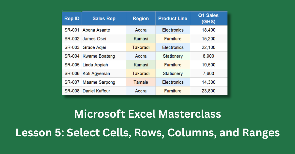
Knowing how to select cells in Excel properly is one of those skills that looks trivial until you realise how much time you’re wasting without it. Most beginners click one cell, drag slowly, and hope for the best. That works for a five-row table. It becomes painful the moment your dataset has thirty rows, twelve columns, and data scattered across multiple sections.
The good news is that selection in Excel follows a consistent logic once you understand it. A handful of techniques covers the vast majority of real work situations. Learn them properly and you’ll move through spreadsheets faster, make fewer accidental edits, and write better formulas from the start.
This post walks through every essential selection method, using a 30-row quarterly sales dataset with reps across four regions — Accra, Kumasi, Takoradi, and Tamale — so every example is grounded in real data you can follow along with.
Quick Takeaways:
- Shift + Click extends your selection from the active cell to wherever you click. No dragging required.
- Ctrl + Click lets you select non-contiguous cells and ranges — hold Ctrl and click anywhere to add items to your selection without losing what you already have.
- Ctrl + Shift + Down selects from your current cell to the last filled cell in that column. It’s the fastest way to grab an entire data column.
- Clicking a column letter or row number selects the entire column or row in one click. Shift + Click selects multiple adjacent ones.
- The Status Bar at the bottom of the screen shows Sum, Average, and Count for any selected range — no formula needed.
How to Select a Single Cell and a Contiguous Range
Start simple. Clicking any cell selects it. The cell address appears in the Name Box on the top left, and the content appears in the formula bar above the grid.
Selecting a Contiguous Range
A contiguous range is a block of connected cells. To select one, click the first cell and drag to the last. For larger ranges, a faster method: click the first cell, then hold Shift and click the last cell. Everything in between highlights instantly.
In the sales dataset, try selecting E3 to H32. That covers all quarterly sales figures for all 30 reps. Click E3, hold Shift, and click H32. The entire block selects without touching the mouse in between. Look at the bottom of the screen — the Status Bar immediately shows the Sum, Average, and Count for that selection. No formula needed. For a quick sanity check on a dataset, this alone saves real time.
Using the Name Box as a Selection Tool
Here’s a shortcut most beginners discover late. Click the Name Box — the small box showing the current cell address above column A — type a range address, and press Enter. Excel selects that range and jumps to it instantly.
Type E3:H32 and press Enter. All four quarters of sales data across all 30 reps highlight in one step. This is especially useful when you need to select a specific range for a formula and the cells are far from each other on a large sheet.
How to Select Entire Columns and Rows
Selecting a full column or row is something you’ll do constantly: applying formatting, inserting data, or running a formula across an entire field.
Selecting a Single Column or Row
Click the column letter at the top of the screen to select the entire column. Click the row number on the left edge to select the entire row. The entire column or row highlights, including every empty cell below or to the right of your data.
In the dataset, click the column header for column E — the Q1 Sales column. All 30 quarterly values highlight. Check the Status Bar. You’ll see the sum of all Q1 sales: GHS 464,100 across the company. That number comes up in one click, no formula typed anywhere.
To select row 8 — the entire record for Daniel Kuffour (SR-008) — click the number 8 on the left side. His full data row highlights: Rep ID, name, region, product line, all four quarters, annual total, target, achievement rate, and rank.
Selecting Multiple Adjacent Columns or Rows
Click the first column letter, hold Shift, and click the last column letter. All columns between them select. The same works for rows.
To select columns E through H — all four quarterly sales columns — click the E header, hold Shift, and click the H header. All four columns highlight together. This is useful before applying consistent number formatting or adjusting column width across multiple columns at once.
How to Select Non-Contiguous Cells and Ranges
This is the technique that separates efficient Excel users from everyone else. Non-contiguous selection lets you select cells or ranges that are not connected — scattered across the sheet — and treat them as one group.
Using Ctrl + Click
Hold Ctrl and click any cell or range. Each click adds to your existing selection without removing what you already have. Release Ctrl and everything you selected remains highlighted.
In the dataset, you might want to compare Naomi Okyere’s quarterly breakdown against the column totals row. Hold Ctrl, click row 15 (Naomi Okyere’s data), then click row 33 (the totals row). Both rows highlight simultaneously. The Status Bar shows combined figures for both selections.
Selecting Non-Contiguous Ranges Across Sections
On the Regional Summary sheet, the sales data is split into four separate blocks — Accra, Kumasi, Takoradi, and Tamale — each with its own headers and totals row. To compare just the Q1 totals across all four regions, you’d normally need four separate lookups. With Ctrl selection, you can highlight all four region total rows at once.
Hold Ctrl, click each region’s total row, and release. The Status Bar shows the combined sum immediately. That’s a cross-region comparison without writing a single formula.
Contextures explains Ctrl selection in detail, including how to use it when building formulas that reference separate ranges.
Keyboard Shortcuts That Make Selection Fast
Mouse-based selection is fine for small ranges. Once your dataset grows past a few hundred rows, keyboard shortcuts become essential.
Ctrl + Shift + Arrow: The Most Useful Selection Shortcut
Place your cursor in E3 — the first Q1 sales value for Abena Asante. Press Ctrl + Shift + Down Arrow. Excel selects from E3 all the way down to E32, the last Q1 value in the dataset. It stops at the last filled cell before any blank. This works in any direction: down, up, left, or right.
This is how professionals select an entire data column without knowing how many rows it contains. You don’t count rows. You let Ctrl + Shift + Arrow find the edge of the data for you.
Ctrl + Shift + End: Selecting the Full Data Block
Click cell A3 — the first cell of actual data in the dataset. Press Ctrl + Shift + End. Excel selects from A3 all the way to the last used cell in the sheet, which in this dataset is L32. The entire data block highlights in one keystroke.
This is particularly useful before copying, formatting, or running analysis on a complete dataset. One shortcut captures everything, regardless of size.
Ctrl + A: Select the Entire Worksheet
Pressing Ctrl + A while your cursor is inside a data range selects the entire contiguous data block first. Press it again and it selects the entire worksheet. This is the fastest way to apply a universal formatting change — font, size, or cell borders — across everything on a sheet.
A practical guide to the full set of Excel selection shortcuts is available at Microsoft’s keyboard shortcuts reference for Excel. It’s worth bookmarking early in your Excel learning.
The Status Bar: Your Instant Selection Calculator
Every time you select a range in Excel, the Status Bar at the bottom of the screen updates automatically. It shows Sum, Average, and Count for whatever is selected — with no formula required.
Select the Annual Total column (column I, rows 3 to 32) in the dataset. The Status Bar immediately shows the sum of all 30 reps’ annual totals: GHS 2,149,000. The average annual performance: GHS 71,633. The count confirms 30 records are selected.
Right-click the Status Bar to customise it. You can add Minimum and Maximum to the display. Once set, those values appear every time you make a selection. I’ve found this particularly useful for quick data validation — selecting a column and immediately checking whether the minimum looks reasonable takes about two seconds and catches outliers before they cause problems downstream.
A Practice Routine That Builds Selection Speed
Open the Quarterly Sales Data sheet from the practice file. Work through these five tasks in order:
Select the entire Q2 column using the column header click. Select only the Accra reps using Ctrl + Click on rows 3, 6, 10, 13, 16, 19, 22, 25, and 29. Select the full data block using Ctrl + Shift + End from cell A3. Select the four quarterly columns together using Shift + Click across column headers E to H. Finally, use the Name Box to jump directly to I3:I32 and check the Annual Total sum in the Status Bar.
Those five tasks cover every major selection technique in practice. Ten minutes of deliberate repetition is worth more than an hour of passive reading.