The first time most people open Excel, they stare at the screen for a few seconds and then start clicking things at random. There’s a lot going on. A grid of cells, a bar full of buttons across the top, tabs lined up like a filing cabinet, and a row of tiny icons that may as well be hieroglyphics until you know what they do.
Learning to navigate the Excel interface properly is the step that makes everything else easier. Once you know where things live and why they’re arranged the way they are, you stop hunting for commands and start actually working. It sounds small. The difference in speed and confidence is not.
This guide breaks down every major part of the Excel interface — the ribbon, the tabs, the toolbar, the formula bar, and the parts most tutorials skip entirely. By the end, you’ll know exactly where to look for any command Excel has to offer.
Quick Takeaways:
- The ribbon is Excel’s command centre — everything is organized into tabs, and each tab groups related commands together.
- You can collapse the ribbon with Ctrl + F1 to get more screen space when working with large datasets.
- The Quick Access Toolbar is customizable — add your most-used commands so you never have to dig through tabs.
- The Name Box does more than display your cell address — type any cell reference into it and press Enter to jump there instantly.
- Right-clicking is underrated. Right-click almost anything in Excel — a cell, a tab, the status bar — and you’ll find a shortcut menu with relevant options.
Understanding the Excel Ribbon

When Microsoft redesigned the Office interface back in 2007, they replaced the old dropdown menus with the ribbon. A lot of people hated it at first. Now it’s the standard, and once you understand the logic behind it, it makes sense.
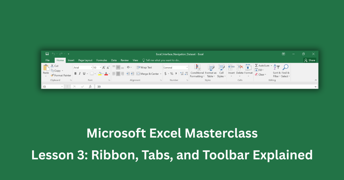
The ribbon sits across the top of the Excel window, just below the title bar. It holds almost every command Excel offers, organised into groups of related tools. The key insight is that the ribbon doesn’t show everything at once — it shows what’s relevant to the tab you’ve selected.
How the Ribbon Is Structured
Each ribbon tab contains groups, and each group contains commands. Take the Home tab as an example. It has groups called Clipboard, Font, Alignment, Number, Styles, Cells, and Editing. Every command inside those groups relates to formatting and basic editing — the things you do most often.
This structure is intentional. Microsoft organized commands by how people actually work, not by what the commands technically do. Once you internalize that logic, finding things becomes much faster.
Collapsing and Expanding the Ribbon
If you’re working on a laptop or a smaller screen, the ribbon takes up real estate. Press Ctrl + F1 to collapse it down to just the tab names. Press it again to bring it back. You can also double-click any tab to toggle it.
I’ve found this particularly useful when reviewing a large dataset and needing to see as many rows as possible at once. One shortcut, and you gain roughly 120 pixels of vertical space.
The Ribbon Tabs Explained

There are eight standard tabs in Excel 2026: Home, Insert, Page Layout, Formulas, Data, Review, View, and Help. A Developer tab also exists but is hidden by default — you can enable it in File > Options > Customize Ribbon.
Home Tab

This is where you’ll spend most of your time as a beginner. It covers copy and paste, font formatting, cell alignment, number formats, and basic editing tools like AutoSum and sorting. If you’re looking for how to make text bold, change a cell colour, or format a number as currency — it’s all here.
Insert Tab

The Insert tab handles everything you add on top of your data — charts, tables, pivot tables, images, shapes, and hyperlinks. When you’re ready to visualize your data, this is the first place to go. Microsoft’s guide to inserting charts in Excel walks through the process step by step.
Formulas Tab

The Formulas tab might be the most valuable one for anyone doing serious analysis. It holds the function library — every formula Excel knows, sorted by category — along with tools for auditing formulas, managing named ranges, and controlling how Excel recalculates. If a formula isn’t working and you don’t know why, the Trace Precedents and Trace Dependents tools in this tab are where you start debugging.
Data Tab

Sorting, filtering, removing duplicates, data validation, importing from external sources — the Data tab handles all of it. Flash Fill, one of Excel’s more impressive features, lives here too. It detects patterns in your data and fills columns automatically based on examples you provide.
View Tab

The View tab controls how you see your workbook rather than what’s in it. Freeze Panes is here — one of the most practical tools for anyone working with a table that has more rows than fit on screen. You’ll also find options to split the window, open the same workbook in two windows simultaneously, and switch between Normal view and Page Layout view.
The Quick Access Toolbar

The Quick Access Toolbar (QAT) sits in the top-left corner of the Excel window, above the ribbon. By default it shows Save, Undo, and Redo. That’s a reasonable start, but it can do a lot more.
Customizing the QAT
Right-click any command anywhere in the ribbon and choose “Add to Quick Access Toolbar.” That command now appears permanently in the top-left corner, one click away regardless of which tab you’re on.
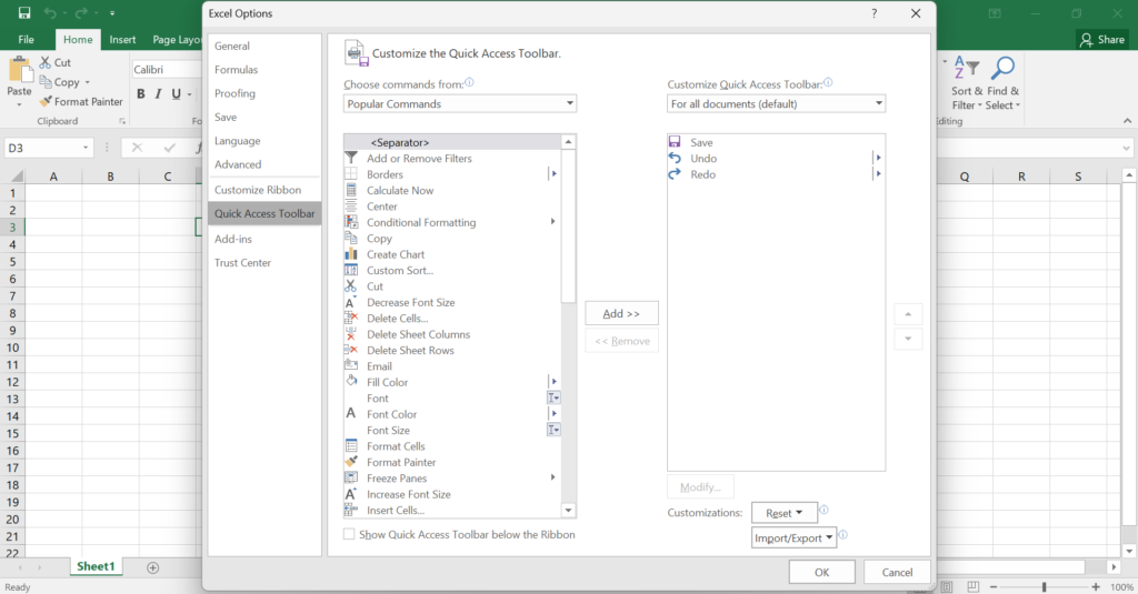
The commands worth adding depend on your workflow. For most people, Print, Freeze Panes, and Format Painter are strong additions. If you run reports regularly, Quick Print saves a surprising amount of time. The goal is to surface the five or six things you do repeatedly and make them available without switching tabs.
The Formula Bar and Name Box
These two elements sit just above the grid and are easy to overlook. They’re more useful than they look.
The Formula Bar

The formula bar shows the actual content of the active cell — the raw formula or value, not the formatted result. If a cell shows “$1,250.00” but you want to see whether that’s a hardcoded number or a formula, click the cell and look at the formula bar. It won’t lie to you.
You can also edit cell content directly in the formula bar. For long formulas, this is often cleaner than editing inside the cell itself.
The Name Box
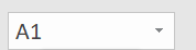
The Name Box is the small box to the left of the formula bar that displays the current cell address — “B4,” for example. Most beginners treat it as a display only. It’s actually a navigation tool.
Click the Name Box, type any cell address or named range, and press Enter. Excel jumps there instantly. Typing “A1” and pressing Enter takes you straight to the top of your sheet no matter where you are. For large datasets, this is faster than scrolling.
The Status Bar and Zoom Controls
The status bar runs across the very bottom of the Excel window. It’s easy to ignore. You shouldn’t.
What the Status Bar Shows

Select a range of cells that contains numbers. Look at the bottom of the screen. Excel automatically displays the Sum, Average, and Count of the selected cells — no formula needed. This is useful for quick sanity checks without committing to a formula anywhere in the sheet.
Right-click the status bar to customize what stats it shows. You can add Min, Max, and Numerical Count to the display with one click.
Zoom Controls

The zoom slider sits in the bottom-right corner. Dragging it adjusts how much of the sheet is visible on screen. A lower zoom shows more data; a higher zoom makes individual cells easier to read. Ctrl + scroll wheel also adjusts zoom if you prefer using the keyboard. Neither changes how the file prints — zoom is a display setting only.
Worksheet Tabs and Sheet Navigation

At the bottom of the screen, below the grid, you’ll find the sheet tabs. Every workbook starts with one sheet. You can add more by clicking the “+” icon next to the last tab.
Right-clicking a tab opens a menu where you can rename it, change its colour, move it, copy it, or hide it. Colour-coding tabs by category — blue for data, green for summaries, orange for reference sheets — is a simple habit that makes multi-sheet workbooks much easier to navigate.
Keyboard shortcuts for sheets: Ctrl + Page Down moves to the next sheet. Ctrl + Page Up moves to the previous one. For workbooks with many sheets, this is faster than clicking with the mouse.
One Change to Make Right Now
Pick one command you use regularly — Format Painter, Freeze Panes, Print — and add it to your Quick Access Toolbar today. Right-click the command in the ribbon, choose “Add to Quick Access Toolbar,” and you’re done.

That’s it. One small change, immediately useful, takes fifteen seconds. Building fluency with the Excel interface works exactly like this — small habits, added one at a time, until the tool stops feeling like an obstacle and starts feeling like an extension of how you think.
In the next lesson, we’ll move from the interface into the grid itself: how cells, rows, and columns work, and how to select and move around your data efficiently.