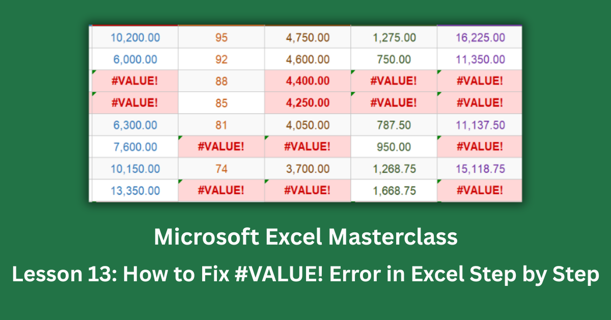
The #VALUE! error is Excel’s way of telling you something is the wrong type. A formula expected a number and got text. It expected a date and got a string that looks like a date but technically isn’t. It tried to add two cells and one of them contained a space character you can’t even see. The error message doesn’t tell you which of these is the problem — it just shows #VALUE! and leaves you to figure it out.
That ambiguity is what makes this error frustrating. Unlike #DIV/0! which always means the same thing, the #VALUE! error can have half a dozen different causes. And because errors cascade in Excel, the cell showing #VALUE! is often not the cell with the actual problem. You fix the wrong place and wonder why nothing changed.
This post walks through every cause of the #VALUE! error in Excel, step by step, using an invoice register dataset where text prices, text dates, and hidden spaces each trigger the error in different columns. By the end, you’ll know how to diagnose which type you’re dealing with and exactly how to fix it.
Quick Takeaways:
- #VALUE! means the wrong data type was used in a formula. The most common cause is a number stored as text — check for left-aligned values in numeric columns.
- A blank-looking cell might contain a space character. That invisible space causes #VALUE! in any formula that uses that cell arithmetically.
- The cell showing #VALUE! is often not where the problem is. Use Formulas tab → Trace Precedents to follow the error back to its source.
- =ISNUMBER(A2) returns FALSE if A2 is text disguised as a number. This is the fastest way to confirm a data type mismatch.
- Fix the root cause, then remove IFERROR. Wrapping an error with IFERROR without fixing the underlying data type problem hides the issue but doesn’t solve it.
What Causes the #VALUE! Error in Excel
The #VALUE! error has one consistent meaning — wrong data type — but several different sources. Knowing which one you’re dealing with before you try to fix anything saves significant time.
Cause 1: Text Stored in a Numeric Cell
This is the most common trigger. A cell looks like it contains a number, but Excel is actually storing it as text. Common examples include prices entered with a currency prefix (“GHS 650” instead of 650), quantities entered with units (“6 units”, “4 pcs”), or numbers imported from another system that came in as text strings.
In the invoice dataset, four invoices have unit prices entered as “GHS 650”, “GHS 340”, and similar. The formula =E*F (price × quantity) immediately produces #VALUE! for those rows because you can’t multiply text by a number.
The easiest way to spot this: look at the cell’s alignment. Numbers right-align by default in Excel. Text left-aligns. If a column of prices has some values leaning left and some leaning right, you have mixed data types. You can also test it directly: =ISNUMBER(E6) returns FALSE if E6 is text disguised as a number.
Cause 2: Text Dates in Date Formulas
Dates are a common source of confusion because they look identical on screen whether they’re stored as true Excel dates or as text strings. The difference shows up the moment you use them in a formula.
In the invoice dataset, five invoices have due dates entered as “15/02/2026” — which Excel treats as plain text, not a date. The formula =TODAY()-D6 (to calculate days overdue) fails with #VALUE! because you can’t subtract a text string from a date.
The telltale sign is alignment again. True Excel dates are right-aligned. Text dates are left-aligned. You can also switch the cell format to General temporarily — a true date shows its serial number (like 46068), while a text date just shows the text string.
Microsoft’s guidance on date storage in Excel explains how the DATEVALUE function converts text dates to true date serials when you can’t re-enter the data manually.
Cause 3: Hidden Space Characters
This one catches experienced users off guard. A cell looks completely blank. Your formula checks it, sees what appears to be nothing, and still produces #VALUE!. The reason: the cell contains a space character. One invisible space. Excel treats it as text, so any arithmetic using that cell fails.
Press F2 on a suspicious empty cell. If your cursor appears to the right of position 1, there’s a hidden character in there. Press Ctrl + A to select all content in the cell, then Delete. Re-enter your value cleanly.
For cleaning a whole column of imported data that may contain spaces, use Find and Replace (Ctrl + H). In the Find field, type a single space. Leave Replace With empty. Click Replace All. Every stray space across the entire column disappears in one step.
Cause 4: Cascading Errors From an Upstream Cell
This is the most common source of confusion when debugging #VALUE!. A formula looks perfectly correct — =G6+I6+J6 — but still shows #VALUE!. Clicking G6 reveals that G6 itself shows #VALUE!. The formula in G6 is the actual problem; your total formula is just an innocent bystander.
Excel errors cascade. When a cell produces #VALUE!, every formula that references that cell inherits the error, even if those downstream formulas are written correctly. Fixing the downstream formulas one by one does nothing. Fix the root cause cell and every downstream formula resolves automatically.
Use the Trace Precedents tool to find the source. Go to the Formulas tab and click Trace Precedents. Blue arrows appear showing exactly which cells your formula reads. Follow those arrows back until you find the cell that originally produced the error.
How to Fix #VALUE! Error in Excel
Fix 1: Clean Text-Formatted Numbers
Option A — Re-enter the value manually. Delete the cell content and type the number without any text characters. Never type currency symbols, unit labels, or other text into cells you plan to calculate with. Apply currency formatting separately via Ctrl + 1 rather than typing “GHS” into the cell.
Option B — Use VALUE() or SUBSTITUTE() in a formula. When you can’t edit the source data (it’s from an external feed, for example), use a formula in a helper column to extract the number:
=VALUE(SUBSTITUTE(E6,”GHS “,””)) strips the “GHS ” prefix and converts the result to a number. You can then use the helper column in your calculations instead of the original cell.
Option C — Text to Columns. Select the column, go to the Data tab, and click Text to Columns. Click Finish without changing any settings. This simple trick forces Excel to re-evaluate the column and often converts text numbers to true numbers in one step.
Fix 2: Correct Text Dates
Option A — Re-enter the date as a true date. Delete the text date and type it in a format Excel recognises: 2026-02-15 or 15-Feb-2026. Before re-entering, format the cell as Date (Ctrl + 1) to confirm Excel will store it correctly.
Option B — Use DATEVALUE(). When you want a formula-based fix rather than re-entering data, =DATEVALUE(“15/02/2026”) converts the text string to a date serial number. You can then use that result in date calculations: =TODAY()-DATEVALUE(D6).
Option C — Use the IFERROR wrapper as a temporary measure. =IFERROR(TODAY()-D6,”Check date”) prevents the error from cascading while you fix the data. Don’t leave it there permanently — it masks future data entry errors.
Fix 3: Remove Hidden Spaces
For individual cells, F2 into the cell and manually delete hidden characters.
For a column of data imported from an external source, a TRIM-based helper column is the cleanest approach. In a blank column, enter =TRIM(A2) for each row. TRIM removes all leading, trailing, and extra internal spaces. Then copy the helper column, use Paste Special to paste as Values only (Ctrl + Alt + V, then V), and delete the original column.
For purely numeric columns, =IFERROR(VALUE(TRIM(A2)),0) handles both the space removal and the text-to-number conversion in one formula.
Fix 4: Handle Array Size Mismatches
Array formulas that multiply or operate on two ranges require both ranges to have the same dimensions. =SUM(A1:A10*B1:B5) fails because one range has 10 rows and the other has 5.
The fix is to make both ranges the same size. If you genuinely have different-sized ranges and need to multiply them, SUMPRODUCT with an IF pad is one option: =SUMPRODUCT(A1:A5,B1:B5) restricted to the shorter range. Or restructure the data so both columns have the same number of rows.
The Fastest Diagnostic Process
When you hit a #VALUE! error, work through this sequence:
Click the error cell and read the formula bar. Identify each cell reference in the formula. Click each referenced cell and check its alignment — left means text, right means number or date. Run =ISNUMBER(cellref) on any suspicious cells. Use Trace Precedents to find upstream errors before assuming the problem is in the formula you’re looking at.
Once you’ve found the root cell, decide whether to fix the data (preferable) or use a formula workaround. Fix the data when you control the source. Use VALUE(), DATEVALUE(), or TRIM() when the data comes from an external system you can’t change.
I’ve found that the most common mistake people make is wrapping a #VALUE! error with IFERROR and calling it done. That makes the spreadsheet look clean but leaves a data quality problem silently ticking underneath. Fix the type mismatch — the fix takes thirty seconds and the spreadsheet actually works correctly afterward.
Open the practice file’s error sheet and work through the broken rows using the diagnostic steps above. The Fixed sheet shows every correction applied, and the Causes and Solutions reference tab maps each scenario to its exact fix formula.