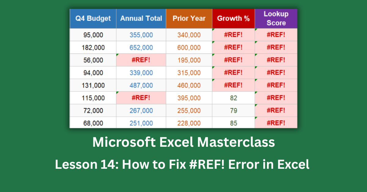
The #REF! error is Excel’s way of telling you a formula is pointing at something that no longer exists. A cell you deleted. A column that got removed. A VLOOKUP that’s trying to return column 6 from a 4-column table. Whatever the cause, the formula’s reference has become invalid — and until you fix it, the calculation simply won’t work.
What makes #REF! different from most Excel errors is how it spreads. Delete one column that several formulas depend on, and every single one of those formulas instantly shows #REF!. Then any formulas that reference those formulas inherit the error too. A single deletion can cascade across dozens of cells in seconds. That speed is both how the error appears and how you know something structural went wrong.
This post covers the four most common causes of the #REF! error in Excel, with specific step-by-step fixes for each one. The examples come from a 20-department budget dataset where deleted rows, VLOOKUP column mismatches, and deleted columns each produce a different version of the error.
Quick Takeaways:
- If #REF! appears inside your formula (like =SUM(C3:#REF!)), a row or column that the formula referenced was deleted. Ctrl + Z is the fastest fix if the deletion just happened.
- VLOOKUP #REF! is almost always a col_index problem. Count the columns in your lookup range and make sure col_index doesn’t exceed that number.
- The cell showing #REF! is rarely where the problem started. Use Formulas → Trace Precedents to follow the chain back to the original broken reference.
- Before deleting any row or column, run Trace Dependents first. It shows you every formula that references the selection — so you can update them before anything breaks.
- Switching from VLOOKUP to XLOOKUP eliminates the col_index #REF! error entirely. XLOOKUP references the return column directly, with no counting required.
What the #REF! Error Actually Means
#REF! stands for reference error. It means the formula contains a cell address that Excel can no longer locate. Sometimes that address appears literally in the formula bar as #REF! — you’ll see something like =SUM(C3:#REF!) rather than =SUM(C3:F3). Other times the formula looks correct but the cell it points to was deleted or moved out of reach.
The error is immediate. The moment you delete a row or column that a formula references, every dependent formula updates to show #REF! in real time. There’s no delay, no warning before the fact.
How to Fix the #REF! Error in Excel: The Four Main Causes
Cause 1: A Deleted Row or Column
This is the most common trigger. You deleted a row as part of a cleanup, or removed a column you thought was unused, and suddenly formulas elsewhere are showing #REF!.
When this happens, the formula bar gives it away. Click the #REF! cell and look. If you see the literal text #REF! inside the formula itself — like =D5+#REF!+F5 — a referenced cell was deleted and Excel has no way to resolve where it pointed.
Fix: Ctrl + Z immediately. If the deletion just happened, pressing Ctrl + Z restores the deleted row or column and the formulas return to normal. This is always the first step.
Fix: Rewrite the formula manually. If Ctrl + Z is no longer available (you’ve made other changes since, or you closed and reopened the file), click the cell, go to the formula bar, and manually replace #REF! with the correct cell address. If the whole column was deleted and the data is gone, you’ll need to recreate that data first.
In the budget dataset, column J (Growth %) shows #REF! on all 20 rows because it referenced a prior year column that was deleted. Every single growth formula broke simultaneously. Recreating the prior year column and rewriting the formula as =IFERROR(G/H-1,”N/A”) restores all 20 rows at once.
Cause 2: VLOOKUP col_index Exceeds the Table Width
This is the second most common source of #REF!, and it’s entirely formula-based. The data is fine. The deletion didn’t happen. The problem is a number in the formula itself.
VLOOKUP’s third argument is col_index_num — it tells Excel which column of the lookup table to return. If you write =VLOOKUP(A4,$M$4:$P$23,5,0) but the range $M$4:$P$23 only spans four columns (M, N, O, P), Excel can’t return column 5. It shows #REF!.
Fix: Count your columns. Select the lookup range and look at the column letters. $M$4:$P$23 spans M, N, O, P — that’s four columns. The col_index must be between 1 and 4. Change 5 to 4 and the error resolves immediately.
In the budget dataset, column I shows #REF! for the first five departments because col_index=5 was used on a four-column lookup table. Changing it to 4 fixes every affected row.
Better fix: Switch to XLOOKUP. Excel 365 and Excel 2019 both support XLOOKUP, which references the return column directly: =XLOOKUP(A4,$M$4:$M$23,$P$4:$P$23). There’s no col_index to count. The column mismatch #REF! becomes impossible. Microsoft’s XLOOKUP documentation covers the full syntax and why it’s the recommended replacement for VLOOKUP.
Cause 3: Out-of-Bounds Relative Reference When Copying
Relative references in formulas shift automatically when you copy them to a new location. That’s useful, but it creates problems near the edges of a dataset.
Imagine a formula in row 3 that reads =B3-A3. Copy it up to row 1 and it becomes =B1-A0. Row 0 doesn’t exist in Excel. The reference is now outside the bounds of the spreadsheet, and #REF! appears.
In the budget dataset, column H (Prior Year) shows #REF! in rows 14 to 18 because a relative reference formula was copied too far in a direction that pushed one of its references out of bounds.
Fix: Delete the out-of-bounds cells. These cells simply don’t need a formula. If the formula makes no sense at that row position, select those cells and press Delete to clear the contents.
Fix: Use absolute references where appropriate. If the formula should always point to the same cell regardless of where it’s copied, add dollar signs. Press F4 while inside a formula to cycle through reference types: A1 becomes $A$1 (fully absolute), then A$1 (row locked), then $A1 (column locked), then back to A1. For a reference that should never shift, use $A$1.
Fix: Add an IF guard. =IF(ROW()>1,B1-A1,0) prevents the formula from running in the first row where the reference would be invalid. This is cleaner than leaving blank rows or relying on structural assumptions about the data.
Cause 4: Named Range Pointing to Deleted Cells
This is the hardest to find because the problem is invisible in the formula bar. A formula like =SUM(AnnualBudget) looks completely valid. But if the cells that the named range “AnnualBudget” points to were deleted, the name itself is broken — and every formula using it shows #REF!.
How to find it: Go to the Formulas tab and click Name Manager. Look at the “Refers To” column. If any named range shows #REF! instead of a cell address, that’s your broken reference. Click the name, click Edit, and update the “Refers To” field to point to the correct cells.
How to Stop #REF! Errors Before They Happen
The Trace Dependents tool is the single most useful prevention step. Before you delete any row or column, select it, go to the Formulas tab, and click Trace Dependents. Blue arrows appear pointing from your selection to every formula that references it.
If arrows appear, don’t delete yet. Update those formulas first, or restructure so they don’t depend on the cells you want to remove. Then delete safely. This takes an extra thirty seconds and prevents errors that can take twenty minutes to untangle.
The second prevention habit: use absolute references ($A$1) for any formula that should point to a fixed cell regardless of where it’s copied. Relative references (A1) are powerful but they shift on copy — sometimes into territory that doesn’t exist.
I’ve found that the most damaging #REF! situations happen when someone reorganises a shared workbook without realising how many formulas depend on its structure. The budget dataset demonstrates this perfectly: deleting one prior year column broke all 20 growth formulas simultaneously, across two different sections of the sheet.
A one-minute Trace Dependents check before any deletion would have flagged exactly which formulas needed updating.
The Quick Diagnostic Sequence
When you see #REF!, work through this quickly. Click the error cell. Look at the formula bar — if you see #REF! written inside the formula, a deletion caused it and Ctrl + Z is your first move. If the formula looks correct, check whether it’s VLOOKUP with a col_index number — count the columns in the lookup range and verify the number fits. If neither of those applies, run Trace Precedents to follow the chain back to the original broken cell.
Fix the source cell. Every downstream cell that inherited the error will resolve on its own once the root is corrected.