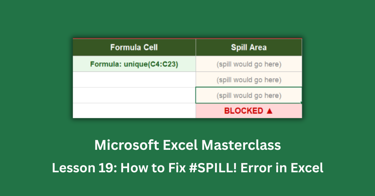
The #SPILL! error is a relatively new addition to Excel’s error family. It arrived alongside dynamic array functions — UNIQUE, SORT, FILTER, SEQUENCE — which were rolled out from Excel 2019 onward and became standard in Microsoft 365. These functions are genuinely useful. They can return multiple results from a single formula, automatically expanding to fill as many cells as needed. But that power comes with a condition: the destination cells must be empty.
When they’re not, you get #SPILL!. The formula is correct. The data is fine. Something is blocking the space where the results need to go. That something could be a value someone typed, a merged cell, the formula being inside an Excel Table, or a range reference too large for the sheet to handle. Each cause has a different fix.
This post works through all six causes of the #SPILL! error in Excel, with step-by-step fixes for each. Examples come from a 20-employee staff performance dataset, where UNIQUE, SORT, and FILTER formulas each encounter different blocking scenarios.
Quick Takeaways:
- #SPILL! means a dynamic array formula can’t fit its results because something is in the way. Click the formula cell and look for the blue dashed border showing where the output needs to go.
- The fastest fix: use the “Select Obstructing Cell” option from the warning icon to jump directly to whatever is blocking the spill.
- Excel Tables and dynamic arrays don’t mix. A UNIQUE or FILTER formula inside a Table column always returns #SPILL! — move the formula outside the Table.
- Never use whole-column references in dynamic array formulas. =UNIQUE(C:C) tries to process over a million rows and almost always causes #SPILL!.
- Merged cells are silent blockers. A merged cell anywhere in the spill path stops the formula completely — unmerge it or use Center Across Selection instead.
Understanding Why #SPILL! Happens
Before 2019, Excel formulas produced exactly one result per cell. One input, one output, one cell. Dynamic arrays changed that. A single =UNIQUE(C4:C23) formula can now return five results — one for each unique department — filling five cells automatically. That automatic expansion is called spilling.
For spilling to work, every cell the output needs to flow into must be completely empty. Not formatted, not containing a formula, not merged — empty. If anything occupies even one of those cells, Excel can’t place the result there and returns #SPILL! instead.
The error itself is Excel being precise, not broken. It’s saying: “I know what the answer is. I just can’t write it anywhere.”
How to Fix #SPILL! Error in Excel
Cause 1: A Non-Empty Cell Is Blocking the Output
This is the most common cause. A value, formula, or even an accidental space character sits somewhere in the cells the dynamic array needs for its results.
Click the cell showing #SPILL!. A blue dashed border appears around the intended spill range — all the cells the formula wants to fill. Scan that range visually. Then click the small yellow warning icon that appears next to the cell. One of the options is “Select Obstructing Cell.” Click it. Excel jumps directly to the blocking cell.
Once you find it, clear it. Press Delete to remove the content. If there’s nothing visible but the spill still fails, try pressing Ctrl + H (Find & Replace), searching for a single space, and replacing with nothing. Invisible space characters are a surprisingly common blocker.
In the staff performance dataset, a =UNIQUE(C4:C23) formula placed in column J tries to spill five unique department names downward. If K8 contains any data at all, the formula returns #SPILL! for all five rows. Remove the content from K8 and all five departments appear immediately.
Cause 2: A Merged Cell in the Spill Path
Merged cells cannot receive spill output. If any cell in the spill range is part of a merged cell block, the formula won’t run.
The tricky thing about this cause is that merged cells don’t always look like they’re in the way. A =SORT(D4:D23) formula tries to sort 20 scores into 20 rows. If cells K16 and K17 are merged somewhere in that range, the sort fails for the entire output — not just those two rows.
Fix: Select the merged cell, go to Home → Merge & Center, and click Unmerge Cells. The formula resolves automatically.
If the merge was purely decorative — centring a heading across columns — use Center Across Selection instead. It looks identical on screen but doesn’t actually merge the cells, so spill formulas can pass through it freely. Find this option in Ctrl + 1, the Alignment tab, under Horizontal alignment.
Microsoft’s guide on merging and unmerging cells covers the Center Across Selection alternative in detail.
Cause 3: The Formula Is Inside an Excel Table
This one surprises a lot of people. If your data is formatted as an Excel Table — the kind with banded rows, automatic filter arrows, and structured references — and you place a dynamic array formula inside one of its columns, you’ll always get #SPILL!. Always.
Excel Tables use structured references that enforce column-by-column logic. Dynamic arrays need to resize their output unpredictably. The two systems conflict by design.
Fix option A: Move the formula outside the Table. Place it in a blank area to the right or below the Table where it has unobstructed space. This is the cleanest solution.
Fix option B: Convert the Table to a plain range. Select any cell in the Table, go to Table Design → Convert to Range, and confirm. The banded formatting disappears but the data stays. The formula now works in the same cell position.
I’ve found option A is usually better in practice. Converting a Table to a range removes the auto-expansion feature that Tables are useful for. Keeping the data in a Table and placing analysis formulas in a separate output area is cleaner architecture.
Cause 4: The Spill Range Extends Beyond the Sheet
Excel worksheets have 1,048,576 rows and 16,384 columns. Any dynamic array formula that tries to produce more results than the available space allows will return #SPILL!.
The clearest example: =SEQUENCE(2000000) asks Excel to generate two million sequential numbers. The sheet doesn’t have two million rows. #SPILL! is the only possible outcome. Less obvious: placing =SORT(A4:A23) in row 1,048,560 leaves only 16 rows below it — not enough to hold 20 sorted values.
Fix: Reduce the output size, or move the formula higher up the sheet where more empty rows exist. For SEQUENCE, use a bounded number: =SEQUENCE(20) instead of =SEQUENCE(2000000). For SORT and UNIQUE, use explicit ranges that match your actual data.
Cause 5: Whole-Column References in Dynamic Array Formulas
A whole-column reference like C:C includes all 1,048,576 rows of column C. When you write =UNIQUE(C:C), Excel tries to evaluate uniqueness across the entire column — including all the empty rows. The output could theoretically reach down for hundreds of thousands of rows, and the formula often runs out of sheet space or memory.
Fix: Use explicit bounded ranges that match your actual data. If your department data runs from C4 to C23, write =UNIQUE(C4:C23). That’s 20 rows of input, returning at most 20 rows of output — manageable and predictable.
For data that grows over time, reference a Table column instead: =UNIQUE(Table1[Department]). Table column references automatically expand to include new rows as data is added, without the overflow risk of a whole-column reference.
Cause 6: Nested Dynamic Arrays With Uncertain Output Size
Combining dynamic array functions can occasionally produce #SPILL! when the intermediate output size can’t be determined before the full formula runs. This is less common in 2026 Excel versions, but can still occur with certain combinations.
A formula like =SORT(FILTER(A4:F23,D4:D23>80)) nests FILTER inside SORT. FILTER’s output depends on how many employees score above 80, which changes with the data. Most current Excel versions handle this fine, but if you encounter #SPILL! from nested arrays, breaking the formula into two steps resolves it reliably.
Place the FILTER result in a helper range first: =FILTER(A4:F23,D4:D23>80). Then reference that helper range in a separate SORT formula: =SORT(helper_range,4,-1). The intermediate step gives Excel a fixed-size input to work with.
Alternatively, the LET function handles this elegantly in a single formula: =LET(filtered,FILTER(A4:F23,D4:D23>80),SORT(filtered,4,-1)). LET evaluates FILTER first, assigns it a name, then passes the named result to SORT. Excel Campus covers the LET function and its uses with dynamic arrays in practical detail.
A Simple Diagnostic Routine for #SPILL!
Click the formula cell. Look for the blue dashed border around the intended output area. Click the warning icon and check what it says is obstructing. If it says “Select Obstructing Cell,” click it and clear whatever is there. If it says “Select Blocking Cell,” you have a merged cell issue.
If the warning points to a Table, move the formula outside. If no specific obstruction is identified, check whether your reference is a whole column and switch it to a bounded range.
Open the practice file’s error demonstration sheet to see each of these causes annotated side by side. The Working Dynamic Arrays sheet shows what each formula looks like when it runs correctly — useful for comparing the difference in setup.