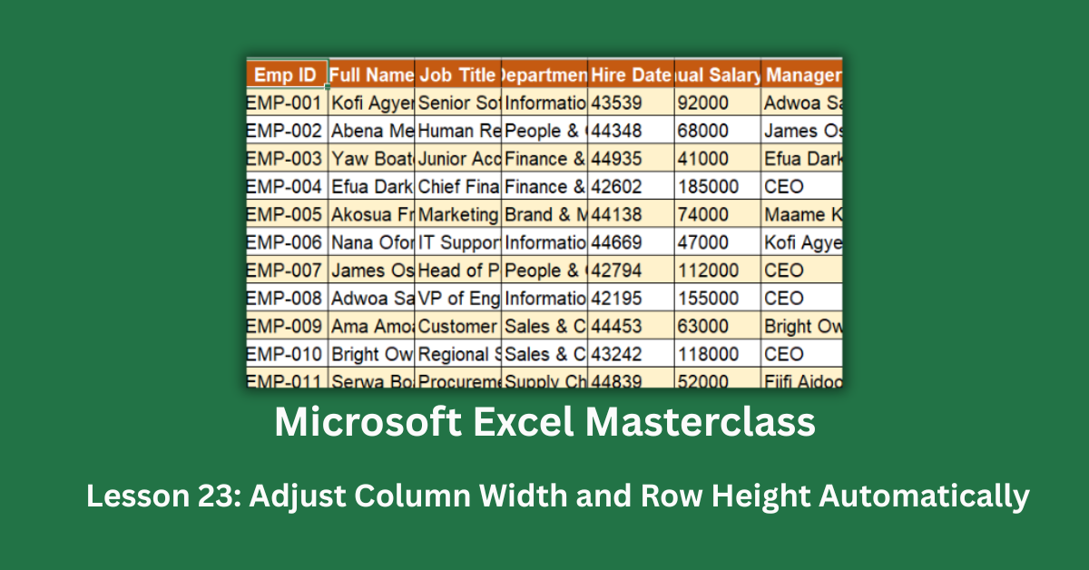
Column width and row height adjustments are some of the most basic formatting tasks in Excel, yet they’re also some of the most frequently done wrong. A spreadsheet where dates show as ##### symbols, employee names are cut off mid-character, and salary figures overflow their cells looks unfinished — and it actively slows down anyone trying to read the data. Getting the sizing right takes less than a minute when you know the right method.
The good news: automatic sizing has been available in Excel since version 2003 and works identically in Excel 2016, 2019, 2021, and all Microsoft 365 builds. Everything covered in this post applies across all modern Excel versions, on both Windows and Mac. The keyboard shortcuts differ slightly between platforms, which is noted where relevant.
This post uses a real employee directory dataset — a 15-person HR register from TechCorp — to show exactly what goes wrong with default column widths and row heights, and how AutoFit resolves every issue cleanly and permanently.
Quick Takeaways:
- Double-click the right edge of any column header to AutoFit that column instantly. No menus required — this single shortcut handles 90% of everyday resizing.
- Select all columns with Ctrl + A, then double-click any column border to AutoFit every column in the sheet simultaneously.
- ##### in a cell always means the column is too narrow to display the value. AutoFit the column and the number or date appears correctly.
- Wrap Text and AutoFit Row Height work together. Enable Wrap Text first, then AutoFit rows to make all content visible without widening columns.
- The keyboard shortcut for AutoFit columns on Windows is Alt + H, O, I. For rows: Alt + H, O, A. Both work from Excel 2007 onward.
Why Column Width and Row Height Matter
Open the RAW_Broken_Layout sheet in the practice file and the problem is immediately visible. Column A (Emp ID) is set to a width of 8.4 — barely wider than the default — while column B holds names like “Kofi Agyeman-Boateng” and “Abena Mensah-Asante” that need significantly more space. Every name in the dataset is cut off. The Hire Date column shows a string of ##### symbols. The Annual Salary column shows numbers without formatting.
The data is all there. It’s just invisible. A report that looks like this tells whoever receives it that no one reviewed it before sending.
Fixing it doesn’t require re-entering data or rebuilding the sheet. AutoFit reads the widest content in each column and resizes to fit it exactly. The same content — correct names, readable dates, properly formatted salaries — appears in seconds.
How to AutoFit Column Width Automatically in Excel
Method 1: Double-Click the Column Border (Fastest)
This is the method worth memorising. Hover over the right edge of any column header letter — the thin vertical line between, say, the B and C headers — until the cursor changes to a double-headed horizontal arrow. Double-click. Excel instantly resizes the column to fit its widest content.
In the TechCorp dataset, column B holds full employee names. “Kofi Agyeman-Boateng” is the longest at 21 characters. After double-clicking the B/C column border, column B widens to exactly accommodate that name. Every name becomes readable in one click.
This works for a single column at a time. For multiple columns at once, select them first, then double-click.
Method 2: AutoFit Multiple Columns at Once
To resize several columns together, select them by clicking the first column header, holding Shift, and clicking the last. Or hold Ctrl and click non-adjacent column headers. Once selected, double-click any of the selected column header borders. All selected columns resize to their individual widest content simultaneously.
To AutoFit every column in the sheet: press Ctrl + A to select all, then double-click any column header border. The FIXED_AutoFit_Layout sheet in the dataset shows the result — column widths ranging from 9 (Emp ID) to 32 (Email Address), each sized to its content rather than a uniform default.
Method 3: Home Tab → Format → AutoFit Column Width
This ribbon method produces the same result as double-clicking. Select the columns you want to resize, go to the Home tab, click Format in the Cells group, and choose AutoFit Column Width. Useful when you’re already working in the ribbon and don’t want to switch to mouse navigation.
Method 4: Keyboard Shortcut (Windows)
Alt + H, O, I — press Alt, then H, then O, then I in sequence (not simultaneously). This navigates the ribbon: Home → Format → Column Width (AutoFit). Select your columns first, then use the shortcut.
On Mac, the ribbon navigation shortcut differs. The most reliable Mac approach is the double-click method or Format → Column → AutoFit Selection from the menu.
Microsoft’s guide to column width in Excel documents all platform-specific options including exact keyboard paths.
How to Adjust Row Height Automatically in Excel
When Row Height Needs Fixing
The RAW_Broken_Layout sheet has all rows set to 15.0 points — the default. That works fine for single-line content. Once Wrap Text is applied to cells with long content, rows need additional height to show the wrapped lines. Without it, only the first line of each cell is visible. The rest is hidden rather than absent.
In the dataset, column H contains office locations like “Headquarters – 3rd Floor, Block B, West Wing.” That text wraps across multiple lines when the column isn’t wide enough to display it in one line. If the row height hasn’t been adjusted, the second and third lines of the address simply disappear visually.
The FIXED_AutoFit_Layout sheet has all data rows set to 51.75 points — enough height to show wrapped text across three lines where needed.
Method 1: Double-Click the Row Border
Hover over the bottom edge of any row number on the left side of the screen until the cursor changes to a double-headed vertical arrow. Double-click. Excel resizes the row to fit the tallest content in that row, including any wrapped text.
Select multiple rows first (click the first row number, hold Shift, click the last) and double-click to resize all of them at once. For every data row in the TechCorp sheet, select rows 2 through 16, then double-click any of the selected row borders.
Method 2: Home Tab → Format → AutoFit Row Height
Select the rows, go to Home → Format → AutoFit Row Height. Identical result to double-clicking, via the ribbon.
Method 3: Keyboard Shortcut (Windows)
Alt + H, O, A for AutoFit Row Height. Select rows first, then use the shortcut sequence.
The Important Catch With Wrap Text
AutoFit Row Height only works correctly when Wrap Text is already enabled on the cells. If Wrap Text is off and long text is overflowing into adjacent cells, AutoFit Row Height will leave the row at its default height because Excel doesn’t consider overflowing text as “wrapped” content.
The correct sequence: apply Wrap Text to the cells first (Home → Wrap Text, or Alt + H, W), then AutoFit the row height. I’ve found that skipping this order is the most common reason people apply AutoFit and then wonder why it didn’t seem to work.
Fixing the ##### Error Specifically
The Sizing_Errors_Reference sheet in the dataset documents five common display problems, and ##### is the first one listed for good reason. It appears in the Hire Date column (column E) and Annual Salary column (column F) on the RAW sheet.
always means the column is too narrow for the value — never that the data is wrong. Dates stored as serial numbers, currency values, large integers — they all show ##### when the column can’t display them.
Double-clicking the column E header border widens the column from its narrow default. The date serial number 43539 becomes 2019-03-15 (Kofi Agyeman-Boateng’s hire date). The value was always there and always correct; the column just wasn’t wide enough to show it.
Setting a Custom Width or Height
AutoFit gives you the exact minimum width or height needed. Sometimes you want slightly more breathing room — padding between the content and the cell border. For that, set a specific value manually.
Right-click any column header → Column Width → type a number. Right-click any row number → Row Height → type a number. For the TechCorp dataset, adding two extra units to each AutoFit width gives a cleaner look without making columns unnecessarily wide.
One Habit Worth Building
Before sharing any Excel file, run a full AutoFit pass. Select all with Ctrl + A, double-click any column header border for columns, then select all rows and double-click any row border. Takes ten seconds. The file arrives looking like someone actually prepared it.
For files you share frequently — weekly reports, monthly trackers — save the properly sized version as your template. AutoFit once, save, and use that file as the starting point for every new version. The TechCorp HR directory in the practice file shows exactly what the difference looks like between the unsized raw version and the AutoFit result.