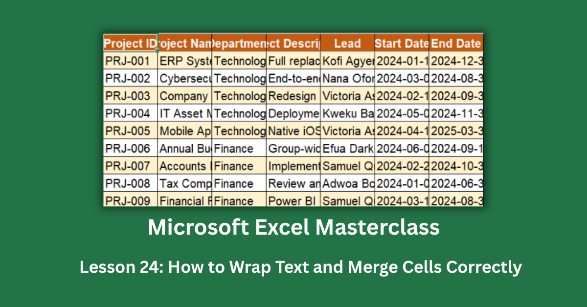
If you’ve ever opened a spreadsheet where a column full of project descriptions looks completely blank, only to discover the content is there — just completely hidden — you’ve felt the frustration of missing wrap text. It’s one of the most common formatting oversights in Excel, and it costs people far more time than it should.
This guide covers how to wrap text and merge cells in Excel the right way, using a real 20-project portfolio report as the working example. You’ll also learn why Merge & Center — one of the most-clicked buttons in Excel — quietly breaks sorting, filtering, and VLOOKUP lookups when used in the wrong place, and what to use instead. These features work in Excel 2016 and all later versions, including Excel 2019, Excel 2021, and Microsoft 365. The “Center Across Selection” alternative covered later is also available across all those versions.
The dataset behind this post tracks 20 active projects across four departments at NexaGroup, with a total portfolio budget of GHS 2,390,000. Without wrap text applied to the description and risk columns, every single project description is invisible. The column headers look fine. The row heights look fine. But the actual content? Gone — hidden past the default 8.43-character column width.
Quick Takeaways:
- Wrap Text alone isn’t enough. You must also AutoFit or manually increase row height, or the text stays clipped below the cell bottom.
- Never merge cells inside a data table. Merge & Center breaks sorting, filtering, and lookup formulas. Use it only for titles and section headers outside the data range.
- “Center Across Selection” is the safer alternative to Merge & Center. It looks identical on screen but leaves every cell independent, so formulas and sorting still work.
- The keyboard shortcut for Wrap Text is Alt + H, W. Use Alt + H, O, A immediately after to AutoFit row heights across your selection.
- Unmerging a merged cell leaves content only in the top-left cell. All other cells in the merged range become blank — there’s no undo for the content loss.
How to Wrap Text in Excel
What Wrap Text Actually Does
Wrap Text tells Excel to fold the content of a cell onto multiple lines within the same cell width, rather than letting it spill across adjacent cells or disappear. Without it, Excel gives you two options: the text overflows into the next empty cell to the right, or it gets cut off at the column boundary if the neighbouring cell has content.
In the NexaGroup project report, the description for PRJ-001 (the ERP System Upgrade) runs to over 200 characters: full platform details, module coverage, integration scope. At the default column width of 8.43 characters, none of that shows. The cell looks empty to anyone who hasn’t clicked into it.
Applying Wrap Text
Select the cells you want to wrap, then go to Home > Alignment > Wrap Text. The keyboard shortcut is Alt + H, W. That’s it for the toggle itself. But here’s where most people stop too early.
Applying Wrap Text does not automatically increase the row height. Excel folds the text visually but keeps the row at whatever height it was when you clicked. If the row was sitting at the default 15pt, your three lines of wrapped text are still showing as one clipped line.
AutoFit Row Height After Wrapping
Right after applying Wrap Text, select your data rows and run Home > Format > AutoFit Row Height (keyboard: Alt + H, O, A). Excel calculates the exact height needed to display all wrapped lines and adjusts each row accordingly. In the formatted version of the NexaGroup report, data rows sit at 90pt height — tall enough to show the full description, risk detail, and milestone text without scrolling inside the cell.
One thing worth knowing: if you later change the column width, row height does not automatically re-adjust. You’ll need to run AutoFit Row Height again. I’ve caught this mistake more than once after resizing a column and wondering why text is suddenly clipped again.
Which Columns Actually Need Wrap Text
Not every column benefits from wrap text. Applying it to date or currency columns in narrow columns creates its own problem: “14-Jun-” appears on line one and “2024” on line two. That looks broken, not helpful.
Wrap Text is appropriate for free-text fields: descriptions, notes, comments, milestones, risk details. In the NexaGroup portfolio report, three columns use wrap text (Project Description at 42 characters wide, Key Risks at 42 characters, and Next Milestone at 36 characters). Every other column stays unwrapped with a width matched to its content.
For a complete reference on Wrap Text options and behaviour, Microsoft’s official Wrap Text documentation covers edge cases including how it interacts with merged cells.
How to Use Merge Cells Correctly in Excel
What Merge & Center Does
Merge & Center combines a selected range of cells into one single cell and centres the content. It’s most commonly used to create report titles that span the full width of a table. In the NexaGroup portfolio report, the title row “NEXAGROUP — PROJECT PORTFOLIO STATUS REPORT | Q2 2024” is merged across all 12 columns. The four department section headers (Technology, Finance, Marketing, HR) are each merged across all 12 columns as coloured banner rows.
That’s exactly the right use for merging. A title above a table. Section separators between data groups. Labels that need to visually span a range without being part of the data itself.
The Right Way to Apply Merge & Center
Select the cells you want to merge, then click Home > Alignment > Merge & Center. You can also use the dropdown arrow next to that button, which gives you additional options: Merge Across (merges each row individually within a multi-row selection), Merge Cells (merges without centering), and Unmerge Cells.
For section headers in the NexaGroup report, each department banner was created by selecting the full row across columns A to M, applying a coloured fill, and then merging. The result is a clearly defined visual group for Technology’s five projects, Finance’s four, Marketing’s four, and HR’s seven.
Where Merge & Center Causes Real Problems
Here’s the honest part that most tutorials skip: Merge & Center is genuinely destructive when used inside a data table. Three specific things break.
Sorting fails. Try to sort a column that contains merged cells and Excel throws an error: “This operation requires the merged cells to be identically sized.” The sort stops entirely.
Filtering fails. AutoFilter can’t process a column where some cells are merged across multiple rows. You get inconsistent or completely wrong filter results.
VLOOKUP and INDEX/MATCH return blanks. A merged cell only stores its value in the top-left cell of the merged range. Every other cell in that range is empty. If you merge cells in a lookup column — for example, merging “Technology” across five rows to label a department group — VLOOKUP finds the correct match for row one and returns blank for rows two through five.
In the NexaGroup portfolio report, the Department column stays fully unmerged in the data table. Each of the 20 rows has its own “Technology”, “Finance”, “Marketing”, or “HR” value. The merged department banners are separate rows inserted between groups — they’re not the data column itself.
The Safer Alternative: Center Across Selection
Why This Option Exists
Center Across Selection is one of Excel’s most underused alignment options. It gives you the exact same visual result as Merge & Center — content appears horizontally centred across multiple columns — but without actually merging the cells. Every cell stays independent.
That means sorting, filtering, VLOOKUP, COUNTIF, and every other formula that references that range still works perfectly.
How to Apply It
Select the cells you want to visually centre across. Press Ctrl + 1 to open the Format Cells dialog. Go to the Alignment tab. In the Horizontal dropdown, choose Center Across Selection. Click OK.
On screen, it looks identical to Merge & Center. But behind the scenes, every cell in that selection retains its own identity. You can click individual cells, reference them in formulas, sort columns, and run filters without any issues.
I’d genuinely recommend using Center Across Selection any time you’re tempted to merge cells inside or near a data range. It eliminates an entire category of headaches.
Formatting Reports with Merge and Wrap Together
How They Work Together in Practice
The NexaGroup portfolio report demonstrates how both tools serve different purposes in the same file. Wrap Text handles the long-form content within the data table — descriptions averaging 150 characters, risk notes running to 180 characters, milestone text at 80 characters. Merge & Center handles the structural framing above and between data groups.
The total portfolio budget of GHS 2,390,000 across 20 projects sits in a merged totals row at the bottom of the report. Average completion across all projects is 53.5% — a figure that only calculates correctly because the % Complete column is unmerged, with a clean decimal value in every row.
Setting Up Print Titles for Merged Headers
One more thing that catches people out: merged title rows only appear on the first printed page by default. If your report prints across multiple pages, page two onwards starts mid-table with no context.
Fix this by going to Page Layout > Print Titles > Rows to repeat at top, then selecting your merged header row and column header row. Every printed page will start with your title and headers. This setting applies per sheet, so you’ll need to configure it separately for each tab in a multi-sheet workbook.
Putting It All Together
The difference between the raw and formatted versions of the NexaGroup report comes down to two decisions applied consistently. Wrap Text on every long-text column, with row heights set to 90pt to match. Merge & Center on title and section header rows only, with every data column left completely unmerged.
Start with your column structure. Get your widths right first. Then apply wrap text to text-heavy columns and run AutoFit Row Height. Add your merged title and section headers last. That order matters: adding columns after you’ve merged headers means re-doing the merge to cover the updated range.
Done in that sequence, the same 20 rows of project data that looked like a blank grid becomes a readable, navigable report where every description, risk, and milestone is fully visible.