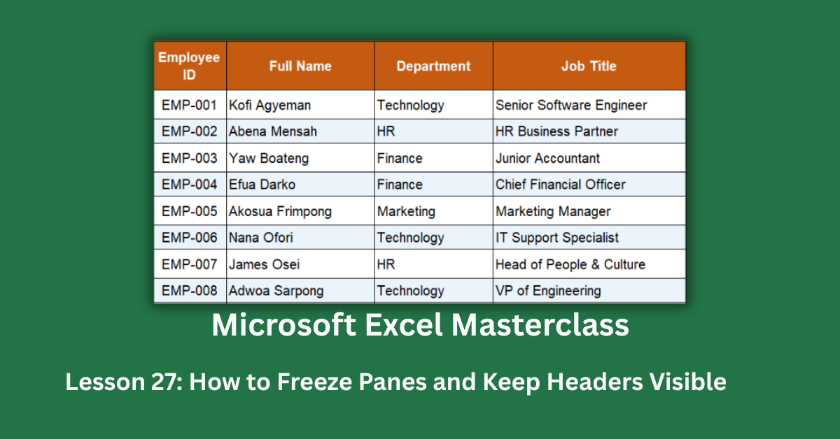
Scrolling down through row 20 of a spreadsheet and suddenly having no idea what the columns mean is one of those small frustrations that adds up fast. You scroll back up, check the headers, scroll back down, and lose your place again. If you’re working with a report that has 28 employees and 16 data columns — like the NexaCorp annual performance dataset behind this guide — that back-and-forth becomes genuinely painful within minutes.
Freeze panes in Excel solve this completely. They lock a section of your spreadsheet in place so it stays visible no matter how far you scroll. This guide covers exactly how to apply them correctly, including the one mistake almost everyone makes with “Freeze Top Row” when their sheet has a title above the actual column headers. These features are available in Excel 2016 and all later versions, including Excel 2019, Excel 2021, and Microsoft 365. The freeze panes behaviour described here is identical across all those versions, including Excel for the web.
The dataset for this guide tracks 28 employees across 6 departments, with 16 columns covering everything from hire dates and salaries ($41,000 to $185,000) to quarterly performance scores, attendance rates, training hours, and annual ratings. Without freeze panes, row 2 — the actual column headers — vanishes the moment you scroll past row 12. Column A (Employee ID) and column B (Full Name) disappear the moment you scroll right past column F. Freeze panes fix both problems with a single setting.
Quick Takeaways:
- The rule for choosing the right freeze cell: select one row below and one column to the right of the last row and column you want to stay visible. For headers in row 2 and key columns A-B, that’s cell C3.
- “Freeze Top Row” locks row 1 only. If your sheet has a title in row 1 and actual headers in row 2, this shortcut freezes the wrong row.
- One freeze pane per sheet. You cannot freeze two separate regions. Applying a second freeze replaces the first.
- Freeze panes do not affect printing. Set Print Titles separately under Page Layout if you want headers on every printed page.
- Double-check after inserting rows above the freeze line. Adding rows above shifts your data down but the freeze stays at its original position, which may now cut into your actual data.
Why Freeze Panes Matter on Wide, Tall Sheets
The scrolling problem in practice
The NexaCorp performance report has 16 columns: Employee ID, Full Name, Department, Job Title, Hire Date, Annual Salary, Q1 through Q4 scores, Annual Rating, Bonus Eligible, Training Hours, Attendance Rate, Leave Days, and Employment Status. That’s a lot of ground to cover horizontally.
When you scroll right to check Q4 scores or attendance rates, columns A and B slide off the left edge of the screen. You can see that someone scored 97 in Q4, but you can’t tell who without scrolling back to the left. With 28 employees earning an average of $80,643 and a total bonus pool of $254,480 on the line, this isn’t a trivial readability problem — it’s a data accuracy risk.
Scrolling down loses your column labels
Scroll down past row 14 in the same sheet and row 2 — the column header row — disappears above the visible area. The numbers are still there. You just can’t tell which one is a Q1 score and which one is a training hour count without scrolling back to the top. Freeze panes eliminate this completely.
How to Freeze Panes in Excel Correctly
The one rule you need to remember
Before you touch the menu, understand this: freeze panes lock everything above and to the left of whatever cell you select. That single rule determines where to click before applying the freeze.
If you want rows 1 and 2 to stay visible, select a cell in row 3. If you also want columns A and B to stay visible, select a cell in column C. Put those together: select cell C3, then go to View > Freeze Panes > Freeze Panes (the third option in the dropdown — not the shortcuts above it). Both rows 1-2 and columns A-B are now locked simultaneously.
Applying the freeze step by step
- Click cell C3 (or whatever cell sits one below and one right of your last fixed row and column).
- Go to the View tab.
- Click Freeze Panes in the Window group.
- Select Freeze Panes from the dropdown (not “Freeze Top Row” or “Freeze First Column”).
A slightly thicker grey line now appears between row 2 and row 3, and between column B and column C. That’s your freeze indicator. Scroll down — rows 1 and 2 stay put. Scroll right — columns A and B stay visible. In the NexaCorp dataset, this means you can scroll all the way to EMP-028’s attendance rate (97.1% average across the team) and still see the employee’s ID, name, and the column label you’re reading.
The Three Most Common Freeze Pane Mistakes
Mistake 1: Using “Freeze Top Row” when headers aren’t in row 1
This is by far the most frequent error, and it catches people who think they’re doing it right. The NexaCorp performance sheet has row 1 as a merged report title: “NEXACORP — ANNUAL EMPLOYEE PERFORMANCE & COMPENSATION REVIEW 2024.” Row 2 contains the actual column headers.
When you click View > Freeze Panes > Freeze Top Row, Excel locks row 1. Only row 1. When you scroll down, the report title stays frozen at the top while the column headers — Employee ID, Full Name, Department, and so on — scroll away with the data. You end up with a frozen title that tells you nothing about the columns you’re reading.
The fix is to ignore the “Freeze Top Row” shortcut entirely. Select cell C3 and use the Freeze Panes option instead. This captures both rows 1 and 2, regardless of whether row 1 is a title or headers.
Mistake 2: Freezing only the first column
Clicking View > Freeze Panes > Freeze First Column locks column A. That keeps Employee IDs visible when scrolling right, which is useful. But it does nothing for vertical scrolling. Scroll down past row 12 and the column headers still disappear, because this shortcut only protects horizontal navigation.
The correct approach handles both directions at once. Cell C3, then Freeze Panes. One selection, one action, both scroll directions covered.
Mistake 3: Selecting the wrong freeze cell
Suppose you’re working in the dataset and you accidentally click cell E5 before applying freeze. Excel locks rows 1 through 4 (including two data rows, which now look like extra headers) and columns A through D. Four columns of fixed content eat up nearly half your visible screen width. The data rows EMP-001 and EMP-002 are now stuck at the top looking like part of the header section.
The fix: go to View > Freeze Panes > Unfreeze Panes first, then reselect C3 and reapply. Always verify your selection before clicking Freeze Panes — one row too many in the freeze is immediately obvious and annoying to undo if you’ve already scrolled deep into the data.
For a complete visual walkthrough of all three wrong positions, Microsoft’s freeze panes documentation includes diagrams showing exactly what gets locked at each cell selection.
Freeze Panes vs. Split View vs. Print Titles
Split is not the same as freeze
Both options sit in the View tab, both draw lines on the sheet, and both get confused regularly. View > Split divides the screen into up to four independently scrollable panels showing the same sheet. Scrolling in one panel doesn’t lock anything in the other — it just creates a second view.
Freeze locks a region in place so it doesn’t scroll at all. For keeping headers visible, freeze is always the right choice. Split is for situations where you need to compare two distant sections of the same sheet simultaneously.
Freeze panes don’t print
Scroll down in the NexaCorp dataset with freeze active. The header row stays perfectly in place. Print the sheet. Page two starts with EMP-013’s data and no column labels at the top.
That’s not a bug. Freeze panes are purely a screen navigation feature. For headers to appear on every printed page, go to Page Layout > Print Titles > Rows to repeat at top, select rows 1:2, and click OK. This is a completely separate setting from freeze, and you need both if you want headers visible both on screen and in print.
One More Thing Worth Knowing
Excel limits you to one freeze pane per sheet. If you try to add a second freeze, the new one replaces the first. There is no way around this.
If you need headers visible across multiple sections of a very long report, convert your data to an Excel Table (Insert > Table). Tables have a built-in behaviour where the column letters at the top of the screen are temporarily replaced with the table’s field names when you scroll within the table bounds. It’s not quite the same as a manual freeze, but it removes the need for one in most cases.
Start with the freeze at C3. Check that both the title row and the header row stay visible as you scroll. Then verify your column names stay readable as you scroll right past the Q4 scores and training hours columns. Done right, you won’t think about freeze panes again until someone sends you a file without them and you have to set it up from scratch.