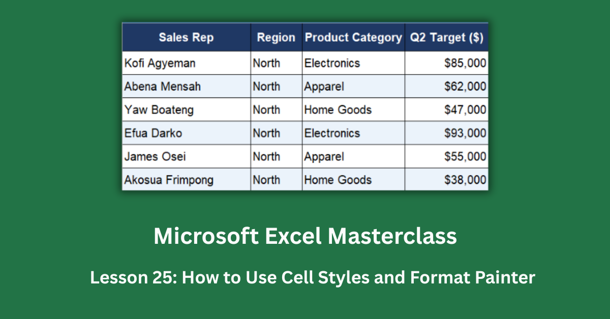
Picture a Q2 regional sales report built by three different people, each handling their own section. The North region heading is Calibri 14pt, bold, blue, underlined. The South heading is Times New Roman 12pt, green, centered. The East heading is Arial 11pt, purple, right-aligned. Same report. Same heading. Three completely different looks. Nobody noticed until it landed in front of the CFO.
That’s the exact dataset behind this guide: 18 sales reps across North, South, and East regions, tracking a $1,096,000 combined Q2 target. The numbers are solid — total actual sales hit $1,099,700, a 100.3% achievement rate. But the formatting tells a story of three people working in isolation with no shared system. Using cell styles and Format Painter in Excel properly fixes exactly this problem, and this guide walks through both tools with real examples drawn directly from that broken report.
These features are available in Excel 2016 and all later versions, including Excel 2019, Excel 2021, and Microsoft 365. Custom cell styles and all Format Painter behaviour described here work identically across those versions. The built-in Good, Bad, and Neutral styles referenced below are also available in Excel for the web, though custom style creation is limited there.
Quick Takeaways:
- Cell styles are workbook-level definitions. Change a style once and every cell using it updates instantly — across every sheet in the file.
- Double-click Format Painter to keep it active across multiple selections. Single-click only paints once, then deactivates.
- Format Painter copies everything: font, fill, borders, number format, and alignment. Always check your source cell before painting to avoid accidentally spreading the wrong number format.
- Use Excel’s built-in Good, Bad, and Neutral styles for performance labels. They use standardised colours that every Excel user recognises, eliminating the risk of reversing red and green.
- Never apply manual formatting on top of a cell style. It partially disconnects the cell from the style, so future style updates stop propagating to that cell.
What Cell Styles Are and Why They Matter
The Problem with Manual Formatting
Every time someone formats a cell manually — picking a font, choosing a fill colour, adjusting the border — that formatting exists only in that cell. It has no memory. The next person who opens the file and adds a new section starts from scratch, picking whatever font they prefer that morning.
In the sales report dataset, this played out across three sections. North’s column headers are Calibri 10pt bold with a light blue fill. South’s are Times New Roman 9pt bold italic with a dark green fill. East’s are Arial 11pt, non-bold, purple, left-aligned. Same eight columns (Sales Rep, Q2 Target, Q2 Actual, Variance, and so on) — three treatments that share nothing visually.
How Cell Styles Solve This
A cell style is a saved formatting definition. You set the font, fill, borders, alignment, and number format once, give it a name, and apply it to cells with a single click. When you need to change the style — say, shifting the header background from navy to dark teal — you modify the style definition and every cell using it updates at the same time.
Excel ships with dozens of built-in styles. Access them via Home > Cell Styles. The gallery groups them by purpose: Titles and Headings, Data and Model, Themed Cell Styles, and Number Format styles. For a sales report, the most useful built-in options are Heading 1 through Heading 4 for section and column headers, and the Total style for summary rows.
Creating a Custom Style
For formatting that the built-in styles don’t cover, you can define your own. Go to Home > Cell Styles > New Cell Style, name it (something like “Section Heading” or “Totals Row”), configure the format settings, and click OK. That style is now available in the Cell Styles gallery for this workbook.
One important caveat worth knowing upfront: custom styles are saved per workbook. If you send the file to a colleague who copies your data into a new workbook, your custom styles don’t travel with it. To share styles across files, use Home > Cell Styles > Merge Styles, which imports styles from another open workbook.
How to Use Cell Styles Correctly in Excel
Applying Built-In Good, Bad, and Neutral Styles
The sales report contains one of the more consequential formatting errors you can make in a performance dashboard. In the North region, the “Exceeded” performance labels have a red fill and the “Below” labels have a green fill — directly reversed from what they should mean. Someone manually assigned the colours and got them backwards. Nothing in the file flags this as wrong.
Excel’s built-in Good, Bad, and Neutral cell styles eliminate this risk entirely. Good is always green. Bad is always red. Neutral is always yellow. They live under Home > Cell Styles > Data and Model. Select your performance label cells, click the appropriate style, done. No colour picking, no chance of reversal.
Eight of the 18 reps in the dataset have “Exceeded” labels. Seven are “Below.” Three hit their targets exactly. In the corrected (styled) version of the report, every single one of those labels uses the appropriate built-in style, and the visual meaning is immediately clear to anyone who’s ever used Excel.
Applying Heading and Total Styles Consistently
The North Totals row carries another problem: it has the same light blue fill as the column headers above it. Someone used Format Painter to copy formatting from a header cell onto the totals row by mistake. The totals look like a second header row, not a summary.
Excel’s built-in Total style (under Titles and Headings in the Cell Styles gallery) applies a bold font with a top border — clear, professional, and universally understood as a summary row. Apply it to all three regional totals rows (North, South, East) and the Grand Total row using the same single click. The Grand Total row in the raw dataset currently uses a garish bright yellow background (#FFFF00) with Calibri 12pt bold — the fourth different style in a report that should have one.
For more on the full Cell Styles gallery and what each built-in style is designed for, Microsoft’s cell styles documentation covers every option available.
How to Use Format Painter Correctly in Excel
The Single-Click vs. Double-Click Difference
Format Painter is the paintbrush icon in Home > Clipboard. It copies all formatting from one cell and pastes it onto another. Most people know the basic version: click the icon, click the target cell, done.
What far fewer people know is that a single click only paints once. The painter deactivates the moment you click your target. If you have three totals rows across three regions to format, a single-click means three separate trips back to the source cell — and three opportunities for the formatting to drift slightly between attempts.
Double-clicking Format Painter locks it on. The paintbrush cursor persists. Click or drag across as many targets as you need. Press Escape when you’re finished. In the dataset, the correct workflow for standardising all three regional header rows would be: select one correctly-formatted header → double-click Format Painter → click each of the other header rows → Esc.
What Format Painter Actually Copies
This is the part that catches people out. Format Painter does not just copy the visible colour and font. It copies every format attribute on the source cell: font family, size, bold/italic/underline, fill colour, border style, horizontal and vertical alignment, and the number format.
In the sales dataset, the South region uses “GHS #,##0” as its currency format — a non-standard prefix typed manually instead of using a proper currency code. If someone selected a South Actual cell as their Format Painter source and painted it over North or East cells, those cells would inherit the GHS format. The numbers would still be correct, but they’d now display GHS 91,200 instead of $91,200.
Always click into the source cell and press Ctrl+1 to check its number format before painting. One second of verification prevents a formatting error spreading across hundreds of cells.
The Manual Override Problem
One last scenario from the dataset’s error reference is worth flagging because it’s genuinely surprising. If you apply a cell style to a cell and then manually format one attribute — say, pressing Ctrl+B to add bold on top of a style that doesn’t include bold — that manual formatting partially disconnects the cell from the style.
Later, if you modify the style to change the font, the manually-bolded cell won’t fully update. The manual attribute takes priority. You end up with cells that look like they’re using the same style but are quietly different underneath.
The fix is to reapply the style: select the affected cells, go to Home > Cell Styles, and click the style again. This reapplies it fresh and clears any manual overrides. The trade-off is that it removes all manual formatting from those cells, so if any of that was intentional, you’ll need a custom style instead.
Putting Both Tools Together
The styled version of the NexaGroup sales report uses four styles applied consistently across all three regions: a Section Heading style for the regional title rows, a Column Header style for the eight-column headers, the built-in Good/Bad/Neutral styles for the performance labels, and a Total style for every summary row. Format Painter was used to carry the column header and data row styles across sections after the first region was set up correctly.
The result is a report where the data does the talking. North exceeded its $380,000 target by $5,050. South beat its $356,000 target by $2,200. East came in $3,550 under its $360,000 target — the only region that missed. Electronics led product performance at 102.0% achievement. Those insights are visible in seconds because the formatting is consistent and the colour coding is correct.
Start with one section. Get every style right. Then use double-click Format Painter to carry that formatting to the rest of the workbook. It takes less time than manually formatting each section, and it produces a result that holds together even when someone else opens the file six months from now.