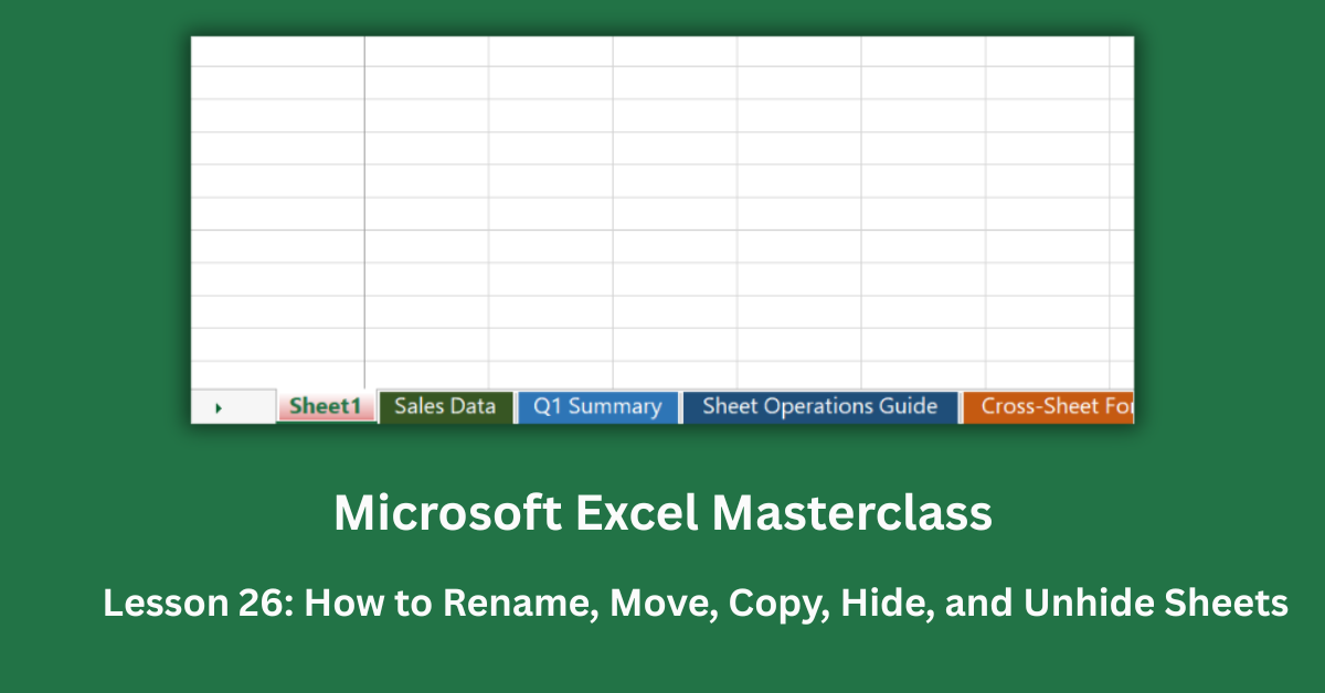
A workbook named “Sheet1, Sheet2, Sheet3” tells you absolutely nothing. Open it six months later and you’re clicking through tabs trying to figure out which one holds the sales figures and which one you accidentally left blank. The NexaCorp workbook behind this guide has seven sheets built around regional sales data — five regions, GHS 8,521,000 in annual revenue, and a hidden employee directory containing 12 staff records with salaries ranging from GHS 42,000 to GHS 96,000. Without proper sheet management, navigating a file like that is a guessing game.
Knowing how to rename, move, copy, hide, and unhide sheets in Excel is one of those foundational skills that pays off every time you open a multi-sheet workbook. Every operation here is available in Excel 2016 and all later versions, including Excel 2019, Excel 2021, and Microsoft 365. Hiding, unhiding, and tab colour features are also available in Excel for the web, though the “Very Hidden” sheet state (covered below) requires the desktop version.
Quick Takeaways:
- Double-click a sheet tab to rename it — the fastest method. Sheet names can’t exceed 31 characters or contain / \ ? * [ ].
- Hold Ctrl and drag a tab to copy a sheet. No dialog needed. Rename the copy immediately — it defaults to “SheetName (2)”.
- Hidden sheets are not secure. Anyone can unhide them with two clicks. For sensitive data like budget figures, use workbook encryption (File › Info › Protect Workbook).
- “Very Hidden” sheets set via VBA do not appear in the Unhide dialog at all. They require a VBA command to restore.
- Moving a sheet to a different workbook removes it from the source file. Use “Create a copy” in the dialog if you want it in both places.
How to Rename Sheets in Excel
The fastest way: double-click the tab
Double-click any sheet tab and the name becomes editable immediately. Type the new name and press Enter. That’s it.
The right-click method (right-click › Rename) does the same thing in two steps. There’s also a ribbon path — Home › Format › Rename Sheet — but unless you already know the keyboard shortcut (Alt + H, O, R), the double-click wins on speed every time.
In the NexaCorp workbook, the first sheet is deliberately left as “Sheet1” to demonstrate the problem. The second sheet, “Sales Data”, shows what it should look like after renaming. Both contain identical regional figures — Accra at GHS 2,887,000, Kumasi at GHS 2,020,000, Takoradi at GHS 1,415,000 — but only one makes sense at a glance.
Naming rules worth knowing
Sheet names have a 31-character limit, which is more than enough for clear names like “Q1 Regional Sales” or “Budget Confidential.” The characters you can’t use are: / \ ? * [ ] and the colon :. Spaces are allowed, but in formulas, a sheet name with spaces needs single quotes around it: =’Sales Data’!A1. Names without spaces are cleaner to reference in formulas.
Renaming updates cross-sheet formulas automatically
This is the part that surprises people. The NexaCorp workbook has a dedicated “Cross-Sheet Formulas” sheet pulling data from “Sales Data” — including Accra’s annual total (GHS 2,887,000) and the Q1 total across all regions (GHS 1,706,000). If you rename “Sales Data” to “Regional Sales 2024”, every formula referencing it updates automatically in the same session. No broken references, no manual fixing.
The risk is renaming a sheet in one workbook that another file references externally. External links use the file path and sheet name — rename the sheet and those external references break immediately. For the full behaviour of cross-sheet references during renaming, Microsoft’s documentation on formula references across sheets covers the edge cases.
How to Move and Copy Sheets in Excel
Moving a sheet by dragging
Click and hold a sheet tab, then drag it left or right along the tab bar. A small black triangle appears showing where the sheet will land when you release. This is the fastest way to reorder tabs in a tidy workbook.
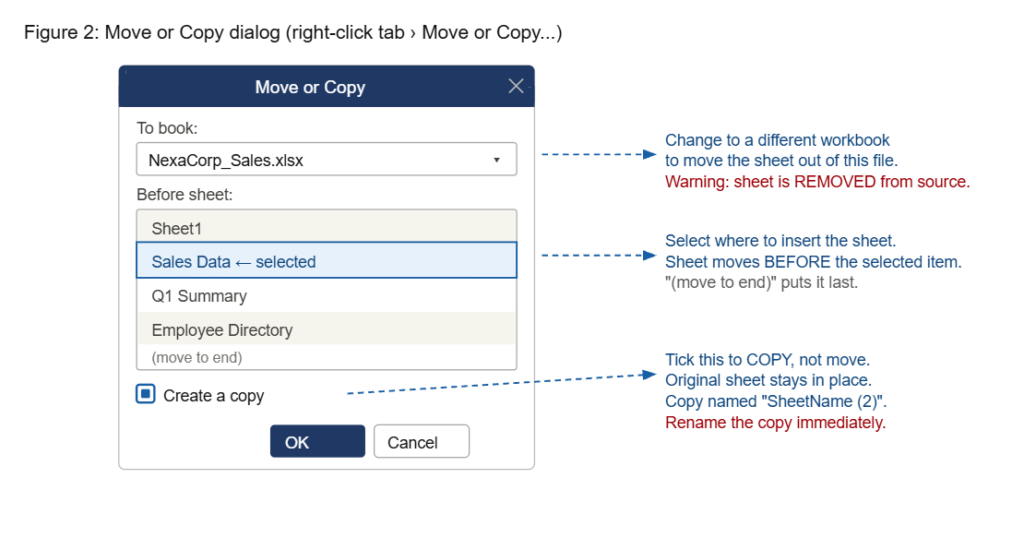
For more precision — or when dragging across many tabs — use the right-click dialog: right-click the tab › Move or Copy › choose where to place it under “Before sheet” › click OK. The “Before sheet” list shows every sheet in the workbook. “(Move to end)” puts it last.
Copying a sheet: Ctrl+drag
Hold Ctrl, then click and drag the tab to a new position. A small “+” appears on the cursor to confirm you’re copying, not moving. Release at the target position and an exact duplicate appears.
The NexaCorp workbook includes a “Q1 Summary” sheet copied from “Sales Data” and trimmed to January through March only, with headcount and revenue-per-head columns added. Accra’s Q1 total was GHS 588,000 against 42 staff, giving GHS 14,000 revenue per head. The copy was created in seconds using Ctrl+drag, then the month columns were updated.
Rename copies immediately. The default name “SheetName (2)” is ambiguous and causes formula confusion fast, especially if you then copy the copy and end up with “SheetName (2) (2).”
Moving a sheet to a different workbook
In the Move or Copy dialog, the “To book” dropdown lets you select any currently open workbook as the destination. This moves the sheet out of its source file permanently. If you want the sheet in both files, tick “Create a copy” before clicking OK.
I’ve seen this catch people when they’re building a summary workbook by pulling sheets from multiple project files. Moving instead of copying silently deletes the sheet from the original, which only becomes obvious when a formula elsewhere throws a #REF! error. Tick the copy checkbox first.
How to Hide and Unhide Sheets in Excel
Hiding a sheet
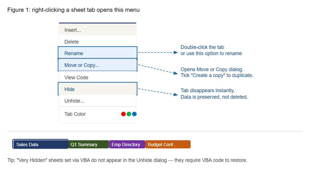
Right-click the tab › Hide. The tab disappears. All data, formulas, and formatting on that sheet remain completely intact — nothing is deleted. Other sheets can still reference data on a hidden sheet, and those formulas continue to return correct values.
The NexaCorp workbook hides two sheets by default. “Employee Directory” contains 12 staff records — roles, hire dates, salaries, and reporting lines. “Budget Confidential” holds the annual budget targets by region, totalling GHS 7,338,000. Both are hidden so they don’t clutter the tab bar during normal use.
One hard limit: you cannot hide the last visible sheet in a workbook. Excel requires at least one sheet to be visible at all times.
Unhiding a sheet
Right-click any visible tab and choose “Unhide.” A dialog appears listing every hidden sheet. Select the one you want and click OK.
The catch: you can only unhide one sheet at a time. If you have five hidden sheets and need to restore all of them, you repeat the process five times. There’s no “unhide all” button in the standard interface. A quick VBA workaround exists for this — For Each ws In Worksheets: ws.Visible = True: Next ws — but for occasional use, the dialog is fine.
The “Very Hidden” sheet — and why it matters
Standard hidden sheets appear in the Unhide dialog. Any user can restore them in two clicks, no password required. This makes hiding suitable for reducing clutter, not protecting sensitive information.
“Very Hidden” is a different state, set only via VBA by changing a sheet’s Visible property to xlSheetVeryHidden. These sheets don’t appear in the Unhide dialog at all. The only way to restore them is via VBA: Sheets(“SheetName”).Visible = True. For workbooks shared externally where certain reference sheets shouldn’t be casually visible, Very Hidden is worth knowing.
For genuinely sensitive data — salary figures, budget targets, personally identifiable information — hiding alone isn’t protection. Use workbook-level encryption: File › Info › Protect Workbook › Encrypt with Password. That prevents the file from opening without a password, which is a different level of security entirely.
Tab Colours and Workbook Organisation
Right-clicking a tab also gives you “Tab Color,” which assigns a colour to the tab. The NexaCorp workbook uses green for “Sales Data,” blue for “Q1 Summary,” and purple for “Employee Directory” (after unhiding it). One subtlety: the active sheet shows only a thin coloured underline at the bottom of the tab. The full colour only becomes visible when you click away to another sheet.
Colour-coding by purpose is more useful than colour-coding by whim. A consistent scheme — green for source data, blue for summaries, orange for work-in-progress, grey for reference sheets — makes a multi-sheet workbook navigable at a glance. Combined with clear naming, it removes the need to click into every tab to understand what a workbook contains.
For a complete walkthrough of workbook and sheet protection options beyond what’s covered here, Microsoft’s guide to protecting sheets and workbooks explains every setting available in the Protect Sheet dialog.
Building Good Workbook Habits
The NexaCorp workbook is built to show the before and after of each operation side by side. “Sheet1” and “Sales Data” carry identical data so you can compare a default-named tab to a properly labelled one. “Q1 Summary” demonstrates a copied-and-trimmed sheet. The two hidden tabs show how hiding keeps a tab bar clean without losing any data.
Start every workbook with names that mean something to anyone who might open it. Rename before you start adding data — cross-sheet formulas will pick up the new name from the start, rather than needing a rename and re-check later. Move sheets into a logical order: source data first, summaries next, reference and configuration sheets last. Hide what you don’t need regularly. Use tab colours to group related sheets visually.
None of these steps takes more than ten seconds individually. Together, they’re the difference between a workbook you open with confidence and one you approach with mild dread.