The NexaSales dataset used throughout this guide has 35 orders, GHS 65,124 in total revenue, and a problem hiding in plain sight: six orders totalling GHS 5,614 are overdue and unpaid. Buried in 35 rows of mixed statuses, those six rows are nearly invisible. Apply a single filter on the Payment Status column and they surface immediately. That’s what filtering does — it doesn’t change your data, it changes what you can see.
Knowing how to filter data in Excel properly is one of the highest-return skills for anyone who works with spreadsheets regularly. It turns a scrolling exercise into a targeted view. This guide covers text filters, number filters, date filters, multi-column filtering, and the one formula mistake that makes your totals look wrong even after a filter is applied. The dataset behind every example is a 35-order sales register spanning five regions and four months of transactions.
All filtering features covered here are available in Excel 2016 and all later versions, including Excel 2019, Excel 2021, and Microsoft 365. Advanced Filter (filter to another location with a criteria range) is also available in those versions. Excel for the web supports basic AutoFilter but has limited Advanced Filter capability compared to the desktop app.
Quick Takeaways:
- Ctrl+Shift+L toggles AutoFilter on and off. Click any cell inside your data first, then press the shortcut. Filter arrows appear on every column header instantly.
- Each active filter column adds an AND condition. If you filter Region = North and Status = Overdue simultaneously, you only see rows where BOTH conditions are true.
- Replace SUM with SUBTOTAL(9,…) for any totals below filtered data. SUM stays at the full dataset total regardless of what the filter shows. SUBTOTAL updates automatically.
- A blank row cuts your filter range in half. AutoFilter stops at the first completely blank row. Rows below it become invisible to the filter entirely.
- Use Alt+; (semicolon) to copy only visible filtered rows. Standard Ctrl+C copies all rows, including hidden ones. Alt+; selects only what’s on screen.
How to Filter Data in Excel: The Basics
Turning on AutoFilter
Click any single cell inside your data range — not a blank cell, not a header cell outside the table, but a cell inside the data itself. Press Ctrl+Shift+L. Filter dropdown arrows appear on every column header row.
That’s the whole setup. From this point, every column header has a dropdown arrow. Clicking it reveals the filter options specific to that column’s data type: text options for text columns, number options for numeric columns, date hierarchy for date columns.
To turn AutoFilter off, press Ctrl+Shift+L again. The arrows disappear and all rows become visible again. Note that this doesn’t clear your filter settings — they’re just hidden. When you re-enable AutoFilter, the previously active filters are still applied.
Filtering by a single column value
Click the dropdown arrow on the Region column. You’ll see a checklist of all five unique values: Central, East, North, South, West. Untick “Select All,” then tick “North” only. Click OK.
The sheet now shows 8 of the 35 orders from the North region, with a combined revenue of GHS 11,075. The row numbers on the left side turn blue to indicate some rows are hidden. The Region column header arrow turns into a funnel icon to signal an active filter.
To clear this filter: click the Region funnel icon and choose “Clear Filter From Region.” Or press Ctrl+Shift+L twice to reset everything.
Text, Number, and Date Filter Options
Text Filters: beyond equals
The basic checklist is fine for exact matches, but Excel’s Text Filters sub-menu offers much more. Click any text column’s dropdown arrow, hover over “Text Filters,” and you’ll see options including Contains, Does Not Contain, Begins With, Ends With, and Custom Filter.
In the NexaSales dataset, filtering the Company column by “Contains: Imports” would instantly pull every company with “Imports” in its name — Crestline Imports, Seabreeze Imports, Cascade Holdings wouldn’t appear, but the importers would. This is faster than building a SEARCH formula for the same job.
Number Filters: isolating ranges and extremes
Click any numeric column’s dropdown, hover over “Number Filters,” and options like Greater Than, Less Than, Between, and Top 10 appear. These are the filters that make financial analysis fast.
Applying “Revenue Greater Than 2,000” to the NexaSales data isolates the high-value orders — Laptop Pros at GHS 4,850 and GHS 9,700, the Smartphone X12 at GHS 9,600, the Digital Camera at GHS 3,920. The low-value office supply and food orders disappear. What was a mixed 35-row register becomes a focused view of premium orders in seconds.
The Top 10 option is particularly useful for ranking. It shows the top or bottom N items by value — top 5 orders by revenue, bottom 10 by delivery time. “10” is the default but you can change it to any number.
One critical point: if a Number column shows “Text Filters” instead of “Number Filters” in the dropdown, at least one cell in that column contains a number stored as text. The ORD-010 order in the RAW sheet has its revenue stored as the text string “2250” rather than the number 2,250. One bad cell disables numeric filtering for the entire column. The fix is selecting that cell, clicking the green triangle warning, and choosing “Convert to Number.”
For a complete reference on every Number Filter option, Microsoft’s filter data documentation covers them all with examples.
Date Filters: by period, not just exact date
Click a date column’s dropdown and hover over “Date Filters.” You’ll see options like This Week, Last Month, This Quarter, Between, Before, and After. These work on real date values — not text-formatted date strings.
Filtering “Order Date Between 01-Jan-2024 and 31-Jan-2024” on the NexaSales dataset returns only January orders, letting you compare Q1 monthly performance without touching a formula. The dropdown also shows a collapsible year/month/day hierarchy if date grouping is enabled.
If Date Filters doesn’t appear and you see “Text Filters” on a date column instead, the dates are stored as text strings. This is exactly what happens with ORD-014 in the RAW sheet, where the order date is stored as “05-Feb-2024” as a string rather than a proper Excel date value. Converting text dates: select the column, go to Data > Text to Columns > Next > Next > Date (DMY) > Finish. Excel converts the strings to real dates and Date Filters becomes available.
Multi-Column Filtering: AND Logic in Action
Every column filter you apply works as an AND condition with every other active filter. Filtering Category = Electronics and then also filtering Revenue > 1,000 shows only orders that satisfy both conditions simultaneously.
In the NexaSales dataset, this combination returns 11 orders — electronics products with order values above GHS 1,000 each. The Bluetooth Speaker (GHS 870) and Wireless Headphones (GHS 660) don’t appear because their revenue falls below the threshold, even though they’re Electronics. Both conditions must be true for a row to show.
The blue funnel icons are your signal that multiple filters are active. I’ve found it easy to forget a filter is active on a column you’re not currently focused on. After a series of filter changes, check every column header for the funnel icon before drawing any conclusions from the visible row count. One hidden filter can make data look significantly different than the full picture.
To clear all active filters without turning AutoFilter off: go to Data > Clear in the ribbon, or Home > Sort & Filter > Clear. This reveals all rows while keeping the filter arrows in place.
The Formula Problem That Breaks Filter Totals
This is the most counterintuitive thing about filtering, and it catches people regularly. You filter your data to show only Overdue orders — 6 rows, GHS 5,614 in revenue. Then you check the SUM formula at the bottom of the Revenue column. It still shows GHS 65,124. The filter is clearly working. The formula hasn’t updated.
SUM() has no awareness of filter state. It calculates across the entire referenced range whether rows are visible or hidden. Every standard Excel function — AVERAGE, COUNT, MAX, MIN — works the same way.
The fix is SUBTOTAL(). Replace =SUM(H3:H37) with =SUBTOTAL(9,H3:H37). The function code 9 tells SUBTOTAL to sum only visible (non-hidden) cells. When you apply or change a filter, the SUBTOTAL result updates immediately. The CLEAN_Ready_to_Filter sheet in the dataset shows both formulas side by side: the blue SUBTOTAL row updates with every filter; the red SUM row stays fixed at GHS 65,124 regardless of what you filter.
SUBTOTAL function codes: 1 = AVERAGE, 2 = COUNT, 3 = COUNTA, 9 = SUM. For filtered analysis, use these instead of their standard counterparts. Microsoft’s SUBTOTAL function reference lists all 11 function codes.
Three Filter Errors Worth Knowing
The blank row trap
The RAW_Sales_Data sheet has a blank row inserted between the South region orders and the East region orders. When AutoFilter is applied, it auto-detects the table range and stops at the blank row. Only the first 12 orders appear in the filter dropdown. The remaining 23 orders — every East, West, and Central order — are invisible to the filter completely.
The fix: delete the blank row before enabling AutoFilter. Or manually select the full data range A2:M37 before clicking Data > Filter, forcing Excel to use your selection rather than auto-detection.
Mixed-case region names create ghost categories
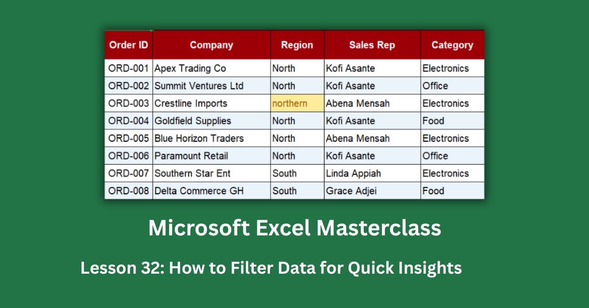
ORD-003 in the RAW sheet has its Region stored as “northern” (all lowercase) instead of “North.” When you open the Region filter dropdown, you see both “North” and “northern” as separate items. Ticking “North” misses ORD-003. You get 7 North orders instead of 8, and the GHS 660 Wireless Headphones order disappears from every North region analysis.
Standardise case before filtering: =PROPER(C3) in a helper column, paste values back, delete the helper. Or Find & Replace: “northern” to “North.”
Copying filtered data brings hidden rows too
Filter to show only the 6 Overdue orders. Select the visible range. Press Ctrl+C. Paste somewhere else. All 35 rows paste, including the 29 hidden ones. Standard copy includes everything in the selection, visible or not.
Press Alt+; (Alt + semicolon) before copying to select only visible cells. Now your paste contains only the 6 filtered rows.
Putting It Together
The GHS 5,614 in overdue revenue across 6 orders becomes actionable the moment you filter for it. South region’s GHS 20,618 total sitting above Central’s GHS 20,434 is a meaningful comparison once you can isolate each region. Electronics accounting for GHS 51,670 out of GHS 65,124 total — nearly 79% of all revenue — is a business insight that doesn’t require a pivot table. It just requires a filter and a SUBTOTAL formula.
Clean your data first. Fix text-numbers, text-dates, and mixed-case fields. Delete blank rows. Then apply filters — and swap your SUM formulas for SUBTOTAL so your totals stay honest.