If you’ve ever stared at a column of numbers and reached for a calculator, the SUM, AVERAGE, COUNT, MIN, and MAX functions in Excel exist precisely for that moment. These five functions are the foundation of almost every spreadsheet analysis — and once you understand how each one thinks, you’ll use them without hesitation.
The good news: all five are available in every version of Excel, including Excel 2013, 2016, 2019, and Microsoft 365. There’s nothing to install or unlock. They work the same way in every version.
Every example here comes from a real dataset: 17 rows of Q1 2024 sales transactions across four salespeople — Ama Owusu, Kofi Mensah, Abena Boateng, and Yaw Asante — selling six products across four regions. That’s the dataset you’ll work through step by step.
Quick Takeaways:
- SUM adds a range of numbers; it silently skips text and blank cells but crashes on error values like #VALUE!.
- AVERAGE divides the total by the count of numeric cells only — blanks don’t drag the average down, but zeros do.
- COUNT only counts cells that contain numbers. Use COUNTA for text, or COUNTIF when you need a condition.
- MIN and MAX ignore text and blanks automatically; a single zero in the range, like a no-stock entry, will become your MIN.
- All five functions use the same syntax pattern: =FUNCTION(range) — master one and the rest feel identical.
What Each Function Is Actually For
Before jumping to syntax, it helps to know what problem each function solves. They’re related, but they answer different questions.
SUM answers: what’s the total? AVERAGE answers: what’s typical? COUNT answers: how many entries do I have? MIN and MAX answer: what are the extremes? Together, they give you a complete statistical picture of any dataset in under a minute.
A Quick Look at the Dataset
The Q1 2024 sales data has 17 rows (Sale IDs S-001 to S-017), but two of those rows contain errors — S-016 has “N/A” in the Units Sold column, and S-017 has “TBD” as the unit price. That gives 15 clean sales records to work with, which matters when you see how each function handles dirty data.
SUM — Add Up a Range Instantly
The syntax is straightforward:
=SUM(H4:H18)
Applied to the Total Sales column, this returns $44,505 across all 15 valid transactions. That’s the Q1 revenue figure in a single formula.
What SUM Skips (and What It Doesn’t)
SUM ignores text cells and blank cells automatically. Kofi Mensah’s S-006 entry shows $0 in Total Sales because he had no stock that day — SUM includes that zero, which is correct. It genuinely was a zero-revenue transaction.
The problem comes with error cells. Rows S-016 and S-017 both show #VALUE! in the Total Sales column. If your SUM range includes those rows, the whole SUM returns #VALUE! too. One error poisons the entire total.
The clean fix is AGGREGATE:
=AGGREGATE(9, 6, H4:H20)
The 9 means SUM, and the 6 tells Excel to ignore error values. Your total stays correct even with broken rows in the range.
AVERAGE — Find the Typical Value
=AVERAGE(G4:G18)
Across the 15 clean rows, the average unit price comes to roughly $421. That figure is skewed upward by laptops priced at $1,200 each — three separate laptop transactions appear in the data. The mouse at $25 sits at the opposite end.
The Zero Problem With AVERAGE
Here’s something worth knowing: AVERAGE skips blank cells but counts zeros. Kofi Mensah’s no-stock entry (S-006) has zero units sold. If you average the Units Sold column, that zero pulls the average down. Whether that’s correct depends on your question.
If you want the average sale size when a sale actually happened, use AVERAGEIF to exclude zeros:
=AVERAGEIF(F4:F18, “>0”, F4:F18)
That’s a subtle but important distinction. I’ve seen reports where a “low average” turned out to be several zero entries dragging the number down — not a real performance problem at all.
COUNT — Know Exactly How Many Records You Have
=COUNT(F4:F18)
Applied to the Units Sold column, this returns 15 — not 17. COUNT skips the two rows where Units Sold contains text (“N/A” in S-016 and a blank). That’s useful: it tells you exactly how many numeric entries you’re working with.
COUNT vs COUNTA vs COUNTIF
This is where most people hit a wall. The three versions work differently:
| Function | Counts | Example Use |
| COUNT | Numeric cells only | How many sales had a unit figure? |
| COUNTA | Any non-empty cell | How many rows have any data at all? |
| COUNTIF | Cells matching a condition | How many sales came from the North? |
For Sale IDs like “S-001” and “S-002” — which are text strings — =COUNT(A4:A18) returns 0. Use =COUNTA(A4:A18) instead and you get 17. That’s a trip-up that’s easy to avoid once you know the rule: COUNT is for numbers only.
MIN and MAX — Spot the Extremes
These two always work as a pair.
=MIN(F4:F18) → 0 (Kofi Mensah, no stock, S-006)
=MAX(F4:F18) → 60 (Yaw Asante, 60 mouse units, S-012)
The range between zero and 60 units tells you immediately how wide the performance spread is. Yaw’s 60-unit mouse sale generated $1,500 in that transaction alone. Kofi’s zero-unit entry generated nothing. Both are real and both belong in the analysis.
MIN and MAX on Price
Switch the range to the Unit Price column:
=MIN(G4:G18) → $25 (Mouse)
=MAX(G4:G18) → $1,200 (Laptop)
That $1,175 price gap explains a lot about revenue variance. A salesperson closing two laptop deals contributes $2,400 before any volume bonus, while the same effort on keyboards nets $110. MIN and MAX surface that gap in two formulas.
Want the second-highest price? =LARGE(G4:G18, 2) returns $350 (Monitor). MIN and MAX only show the extremes — LARGE and SMALL let you step through the ranking.
When These Functions Hit Errors
A few errors come up repeatedly with these five functions:
#VALUE! appears when a text value sits inside a numeric range. The “N/A” in S-016’s Units Sold cell triggers this in formulas that multiply rather than sum. Fix it with IFERROR:
=IFERROR(F4*G4, 0)
#NAME? means Excel doesn’t recognise the function name. =AVARAGE or =SUMT both trigger it. The fix is always the same: start retyping and let autocomplete handle the spelling.
Wrong COUNT is the sneaky one. If you use COUNT on a column of Sale IDs (text), you get zero and assume something’s broken — but COUNT is simply working as designed. Switch to COUNTA.
For any formula that might encounter errors in its range, =AGGREGATE(9, 6, range) for SUM and =AGGREGATE(1, 6, range) for AVERAGE are the safest versions when your data isn’t perfectly clean.
Putting All Five Together
Here’s what a complete summary block looks like for the Q1 dataset, with all five functions working together:
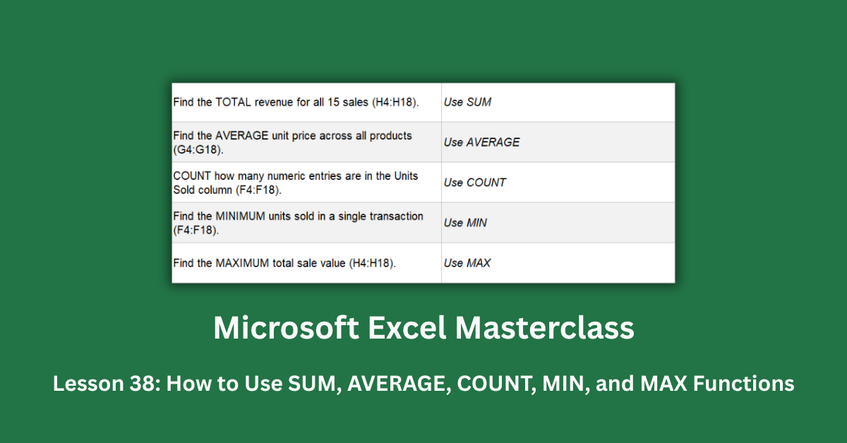
=SUM(H4:H18) → $44,505 total revenue
=AVERAGE(G4:G18) → $421 average unit price
=COUNT(F4:F18) → 15 numeric sales entries
=MIN(F4:F18) → 0 lowest units in a single sale
=MAX(F4:F18) → 60 highest units in a single sale
Five formulas. Five different answers. Together they tell you the total, the typical, the count, and the extremes — which is honestly most of what you need for a sales snapshot.
From here, the natural next steps are conditional versions of the same functions: SUMIF to total by region, AVERAGEIF to average by product, COUNTIF to count by salesperson. Microsoft’s guide to SUMIF and COUNTIF is the clearest starting point. For anyone who wants to go deeper on statistical functions, Chandoo’s Excel function guide covers the full range with worked examples. And ExcelJet’s function reference has a one-page summary of every function you’ll encounter next.
These five functions are the ones you’ll use in almost every spreadsheet you touch. Get them solid, and the rest builds naturally on top.