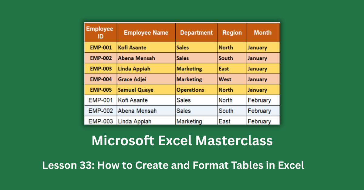
Here’s a scene a lot of people recognize: you open Excel, type in your data — employee names, sales figures, months, departments — and then spend the next 20 minutes manually shading rows, adjusting column widths, and hoping that when you add new data next week, nothing breaks.
Sound familiar?
What most beginners don’t know is that Excel has a built-in feature that handles all of that automatically. It’s called an Excel Table, and pressing just two keys — Ctrl + T — unlocks it instantly.
Excel Tables are not just pretty formatting. They are smart, dynamic, self-updating data containers that make filtering, sorting, calculating, and referencing your data dramatically easier. Once you learn them, you won’t go back.
In this guide, we’re going to walk through everything: how to create a table, how to format it, the most common mistakes that break tables, and how to use powerful features like structured references and the Total Row. We’ll use a real sales dataset — NexaCorp Group’s Q1–Q2 2024 Sales Performance Report — so every example is grounded in something practical.
Let’s get into it.
Quick Reference: Excel Table Features at a Glance
Before we dive into the deep explanation, here’s a summary table so you can jump straight to what you need.
| Feature | What It Does | How to Access It |
| Create Table | Converts a plain data range into a smart Excel Table | Select data → Ctrl + T |
| Table Style | Applies automatic banded color rows and borders | Table Design tab → Table Styles |
| Table Name | Gives your table a meaningful name for formulas | Table Design tab → Table Name box |
| Filter Arrows | Auto-adds dropdown filters to every column header | Added automatically on creation |
| Total Row | Adds a summary row with SUM, AVERAGE, COUNT, etc. | Table Design tab → ☑ Total Row |
| Structured References | Lets formulas reference columns by name, not cell address | Auto-used when you type formulas inside a table |
| Auto-Expand | Table grows when you add data in the next row | Press Tab from the last cell of the last row |
| Calculated Column | One formula fills the entire column automatically | Type a formula in any cell of an empty column |
| Resize Handle | Drag to include or exclude rows/columns | Blue triangle at the bottom-right corner of the table |
Keep this table bookmarked. We’ll explain every row in detail below.
What Exactly Is an Excel Table?
Think of a regular Excel spreadsheet as a whiteboard. You can write anything anywhere, but nothing is connected. An Excel Table, on the other hand, is like a smart form — every row and column knows it belongs together.
Technically, an Excel Table is a named, structured range that Excel treats as a single object. It has:
- A header row with unique column names
- Data rows that are automatically included in sorting, filtering, and formulas
- An optional Total Row for quick calculations
- A name (like SalesData) that you can use in formulas instead of cell addresses like A3:N23
When we converted our NexaCorp dataset into a properly structured table — named SalesData — Excel immediately recognized 20 rows of data across 13 columns tracking employee performance from January to April 2024.
Did You Know? Excel Tables were introduced in Excel 2007. Before that, you had to use something called a “List” which had far fewer features. If you’re on Excel 2007 or newer, you have full Table support.
How to Create an Excel Table (Step by Step)
Step 1: Prepare Your Data
Before you press Ctrl + T, your data needs to be clean. This is the step most beginners skip — and it causes all kinds of headaches later.
Here’s your pre-table checklist:
- Every column must have a unique header in Row 1. No blank headers, no duplicates.
- No merged cells anywhere in your data range.
- No blank rows inside your data.
- No stray data sitting in cells immediately adjacent to your data range.
- Consistent formulas in any calculated columns (no random hardcoded numbers mixed in).
We’ll show you exactly what happens when you violate each of these rules in the Common Mistakes section below. Spoiler: the NexaCorp raw dataset had six of these problems before it was cleaned up.
Step 2: Click Inside Your Data
Click any single cell within your data range. You don’t need to select the whole range — Excel is smart enough to detect the boundaries automatically.
For our NexaCorp data, that means clicking anywhere in the sales table that contained columns like Employee ID, Employee Name, Department, Region, Month, Units Sold, Unit Price (GHS), Revenue (GHS), Target (GHS), and so on.
Step 3: Press Ctrl + T
Hit Ctrl + T (or go to Insert → Table on the ribbon). A small dialog box appears asking you to confirm the table range.
You’ll see something like: “Where is the data for your table? $A$3:$N$23 ✓ My table has headers”
Make sure “My table has headers” is checked, then click OK.
That’s it. Your plain data range is now a proper Excel Table.
Step 4: Give Your Table a Name
By default, Excel names your table something generic like Table1 or Table2. This is fine for small workbooks, but if you ever have multiple tables or write formulas referencing your table, a generic name becomes a nightmare.
Immediately after creating the table:
- Click anywhere inside the table.
- Go to the Table Design tab (it appears in the ribbon when you’re inside a table).
- In the top-left corner, find the Table Name box.
- Delete “Table1” and type a meaningful name — like SalesData.
- Press Enter.
For the NexaCorp dataset, the table was named SalesData. This means instead of writing a formula like =SUM(H4:H23), you can write =SUM(SalesData[Revenue (GHS)]) — which is readable, self-documenting, and automatically adjusts as the table grows.
Pro Tip: Table names cannot contain spaces. Use underscores or CamelCase instead. Sales_Data or SalesData both work. Sales Data does not.
How to Format an Excel Table
Once your table is created, you can control exactly how it looks using Table Styles.
Applying a Table Style
- Click anywhere inside your table.
- Go to the Table Design tab.
- In the Table Styles gallery, hover over any style to see a live preview.
- Click to apply it.
The NexaCorp SalesData table uses Table Style Medium 2 — a clean blue-banded style that makes it easy to read across rows, especially when there are 13 columns side by side.
Styles fall into three categories:
- Light — Minimal shading, mostly borders. Good for printing.
- Medium — Banded color rows with a colored header. Best for screen viewing.
- Dark — Bold header and dark shading. Good for dashboards and presentations.
Banded Rows and Why They Matter
Banded rows (alternating light and slightly darker rows) serve a real purpose — they make it much easier for your eyes to track across a wide row of data without losing your place. When you’re reading Kofi Asante’s January figures across 13 columns, banded rows are the difference between “easy read” and “staring contest.”
The best part: Excel updates the banding automatically when you add or delete rows. You never manually recolor a single row again.
Turning the Total Row On and Off
The Total Row is one of the most useful table features. It adds a dedicated summary row at the bottom of your table.
To enable it:
- Click inside the table.
- Go to Table Design → check the Total Row checkbox.
A new row appears at the bottom. By default, it shows the SUM of the last numeric column. But you can customize each column independently.
To change the aggregate function:
- Click a Total Row cell.
- A dropdown arrow appears.
- Choose: Sum, Average, Count, Max, Min, StdDev, Var, or None.
For the NexaCorp SalesData table, the Total Row shows:
- Total Revenue (GHS): 1,929,200
- Total Units Sold: 943
- Total Commission Paid: 136,060
Quick Win: The Total Row uses SUBTOTAL() formulas internally, not plain SUM(). This is actually smarter — SUBTOTAL() only counts visible rows. So when you filter to show just the Sales department, the Total Row automatically updates to show only Sales totals. Plain SUM() would still show the full total.
Column Width and Row Height
After creating a table, auto-fitting your column widths makes it instantly more readable.
Quick method: Select all columns → double-click any column border in the header row. All columns snap to fit their content.
Keyboard shortcut: Select all with Ctrl + A → Alt + H + O + I to auto-fit column widths.
Understanding Structured References (The Hidden Superpower)
This is the feature that separates beginners from intermediate Excel users.
When you write formulas inside an Excel Table, Excel automatically uses structured references instead of cell addresses. Instead of =F4*G4, Excel writes =[@[Units Sold]]*[@[Unit Price (GHS)]].
These references use the actual column names and are infinitely more readable.
The [@[Column Name]] Syntax
| Reference | What It Means |
| [@[Units Sold]] | The value in the Units Sold column of this row |
| [Revenue (GHS)] | The entire Revenue column of the table |
| SalesData[Revenue (GHS)] | The Revenue column of the SalesData table specifically |
| SalesData[[Units Sold]:[Revenue (GHS)]] | A range of columns from Units Sold to Revenue |
Real Formulas from the NexaCorp Dataset
Here’s how the SalesData table calculates its key columns using structured references:
Revenue calculation:
=[@[Units Sold]]*[@[Unit Price (GHS)]]
This multiplies each employee’s units sold by their unit price to get their monthly revenue.
Commission earned:
=[@[Revenue (GHS)]]*[@[Commission %]]
Applies the commission percentage to that employee’s revenue.
Target achievement:
=[@[Revenue (GHS)]]/[@[Target (GHS)]]
Shows what percentage of the sales target each employee hit.
Totaling the entire Revenue column from outside the table:
=SUM(SalesData[Revenue (GHS)])
You can use this anywhere in the workbook to reference the table’s revenue column.
Counting top performers:
=COUNTIF(SalesData[Performance Rating],”Exceeds”)
Counts how many rows have “Exceeds” in the Performance Rating column.
In the NexaCorp data, this formula returned 16 — meaning 16 out of 20 employee-month records showed performance that exceeded target.
Why Structured References Are Better Than Cell References
Imagine you add 10 more employees next month and the table grows. With regular cell references like =SUM(H4:H23), you’d need to manually update the formula. With =SUM(SalesData[Revenue (GHS)]), the formula automatically includes the new rows. The table adjusts itself.
Pro Tip: Calculated columns in Excel Tables are a game-changer. When you type a formula in one cell of a blank column, Excel automatically fills the same formula into every other row of that column. The whole column becomes consistent instantly. You can see this behavior in action with the Revenue column in the SalesData table — one formula, 20 rows, zero manual copying.
Adding and Removing Rows and Columns
Adding a New Row
The cleanest way to add a row to an Excel Table is to press Tab from the last cell of the last data row. The table auto-expands, applies the banded style, and auto-fills any calculated column formulas.
Alternatively, right-click any row inside the table → Insert → Table Rows Above/Below.
Common mistake: Typing data directly below the last row (outside the table boundary) instead of using Tab. The new data won’t have table formatting, won’t be included in Total Row calculations, and formulas won’t auto-fill.
Adding a New Column
Type a header in the blank cell immediately to the right of the last column header. Excel asks if you want to extend the table — say yes, and the new column is automatically part of the table.
Or: right-click any column header inside the table → Insert → Table Columns to the Left/Right.
Removing Rows or Columns
To delete a row: Right-click the row inside the table → Delete → Table Rows.
Warning: Don’t press the regular Delete key on a selected row — that only clears the cell contents, leaving a blank row that can mess up filters and the Total Row.
Resizing the Table Manually
See the small blue triangle at the bottom-right corner of the table? Drag it to expand or shrink the table range — up or down to add/remove rows, left or right to add/remove columns.
Common Mistakes That Break Excel Tables
This is where most beginners lose hours of their time. The NexaCorp raw dataset (the RAW_Plain_Range sheet) was intentionally built with six real errors so you can see exactly what goes wrong. Let’s walk through each one.
Mistake 1: Merged Cells in the Data Range
What happened in NexaCorp’s raw data: Rows 1 and 2 had merged cells — a merged title row spanning all columns, and a merged sub-header row below it.
What happens when you try Ctrl + T: Excel shows an error: “Cannot create a table that overlaps a merged cell.” The table cannot be created at all until the merge is removed.
Why this happens: Excel Tables require every cell to be completely independent. Merged cells span multiple columns or rows, which breaks the row-by-row structure that Tables depend on for sorting, filtering, and structured references.
How to fix it:
- Select the merged cells.
- Go to Home → Merge & Center dropdown → Unmerge Cells.
- Recreate your title above the table in a completely separate row that sits outside the table range.
Pro Tip: If you want your title to visually appear centered across multiple columns without merging, use “Center Across Selection” instead. Go to Ctrl + 1 → Alignment tab → Horizontal → Center Across Selection. It looks identical to a merge but doesn’t actually merge — and it won’t block your table.
Mistake 2: Duplicate Column Headers
What happened in NexaCorp’s raw data: Both column H and column I were labeled “Revenue (GHS)” — one was actual revenue, the other was the sales target.
What happens: Excel doesn’t reject your table, but it silently renames the second column to “Revenue (GHS)2”. Now any formula using [@[Revenue (GHS)]] only references the first column. Your second column is effectively invisible to your formulas.
How to fix it: Before creating the table, make sure every single column header is unique. Scan for duplicates using:
=COUNTIF($3:$3, C3) > 1
Place this formula next to your header row. If it returns TRUE for any column, you have a duplicate.
In the NexaCorp case, “Revenue (GHS)” in column I was correctly renamed to “Target (GHS)” before the table was created.
Mistake 3: Blank Row Inside the Data
What happened in NexaCorp’s raw data: There was a completely blank row between the February data and the March data.
What happens: When you press Ctrl + T, Excel auto-detects your data range by expanding outward from your selected cell until it hits a blank row or column. The blank row signals the end of the data. Everything below it is excluded from the table — silently, with no warning.
In the NexaCorp case, March and April data (10 rows) were completely left out of the table.
How to fix it:
- Delete the blank row (right-click → Delete Row).
- Then press Ctrl + T. Verify the highlighted range in the dialog box covers all your rows before clicking OK.
Alternative: If you can’t remove the blank row, manually select your full intended range before pressing Ctrl + T. Excel will use your selection instead of auto-detecting.
Mistake 4: Manual Formatting That Fights the Table Style
What happened in NexaCorp’s raw data: Rows 4 through 8 had manually applied gold/orange fill colors and Calibri font formatting applied directly to the cells.
What happens: When you apply a Table Style (like Medium 2), rows 4–8 still show the old gold/orange color instead of the clean blue banding. The table style layers on top of manual formatting, but manual formatting wins.
How to fix it before creating the table:
- Select all data cells.
- Go to Home → Editing → Clear → Clear Formats (the eraser icon dropdown).
- This removes all explicit formatting — fills, fonts, borders — without deleting values.
- Now create the table and apply your style. It applies uniformly to every row.
Caution: Clear Formats also removes number formatting (like currency or date formats). After clearing, reapply any number formats to the relevant columns.
Mistake 5: Hardcoded Value in a Calculated Column
What happened in NexaCorp’s raw data: In the Revenue column (column H), every cell contained the formula =[@[Units Sold]]*[@[Unit Price (GHS)]] — except one cell, H11, which contained the hardcoded number 43,500 instead of a formula.
What happens: Excel detects the inconsistency and flags cell H11 with a green triangle warning: “Formula Inconsistent with Column.” The table column appears to be a calculated column, but this one row won’t update if the Units Sold or Unit Price changes. Your data becomes unreliable.
How to fix it:
- Click the inconsistent cell (H11).
- Click the green triangle warning icon that appears.
- Select “Restore to Calculated Column Formula.”
Excel replaces the hardcoded 43,500 with the correct structured reference formula. The warning disappears.
Mistake 6: Stray Data Adjacent to the Table Range
What happened in NexaCorp’s raw data: Column N contained notes and comments sitting immediately to the right of column M (the last real data column).
What happens: When Ctrl + T auto-detects the table range, it expands in all directions until it hits a blank row or column. Since column N had data adjacent to column M, Excel included column N in the table — creating an unwanted “NOTES” column with a filter arrow and banded formatting.
How to fix it:
- Move the notes column to at least two columns away (e.g., column P), leaving column N blank as a boundary.
- Or delete the notes and add important ones as cell comments (right-click → Insert Comment) on the relevant cells — they stay attached to the cell without affecting the table structure.
After creating the table, verify the range in Table Design tab. It should show A3:M23, not A3:N23.
The NexaCorp Performance Summary: What the Formatted Table Revealed
Once the SalesData table was properly formatted and all errors fixed, the Total Row and structured reference formulas gave us a clean, accurate summary:
| Metric | Value |
| Total Data Rows | 20 (5 employees × 4 months) |
| Total Revenue (GHS) | 1,929,200 |
| Total Commission Paid (GHS) | 136,060 |
| Total Units Sold | 943 |
| Average % of Target Achieved | ~105% |
| “Exceeds Target” Ratings | 16 out of 20 |
| “Meets Target” Ratings | 4 out of 20 |
| Top Earner | Kofi Asante (Sales, North) |
| Highest Month | March — GHS 536,400 total |
None of this was calculated manually. Every figure came from structured reference formulas referencing the SalesData table. As soon as the data was corrected and the table was created, the Summary sheet populated automatically.
That’s the power of a properly structured Excel Table.
Filtering and Sorting Inside a Table
One of the most immediately useful things about an Excel Table is the filter arrows that appear on every column header the moment you create the table.
Filtering Data
Click any filter arrow and you’ll see:
- Sort A to Z / Sort Z to A (or ascending/descending for numbers)
- Text Filters (Contains, Begins With, Equals, etc.)
- Number Filters (Greater Than, Top 10, Between, etc.)
- A checklist of every unique value in the column
For example, clicking the filter arrow on the Department column of the NexaCorp SalesData table shows: Sales, Marketing, Operations. Uncheck “Operations” and “Marketing,” and the table instantly filters to show only Sales department rows. The Total Row updates to reflect only the Sales figures.
To clear a filter: click the filter arrow again → Clear Filter from [Column Name].
Sorting Data
To sort by Revenue from highest to lowest:
- Click the filter arrow on the Revenue column.
- Select Sort Largest to Smallest.
The entire table — all 13 columns — reorders together. Your data stays coherent; you never get the Revenue column sorted while the employee names stay in the original order (a common disaster with non-table data).
Quick Win: To add a secondary sort (e.g., sort by Department first, then by Revenue within each department), go to Data tab → Sort and use the multi-level sort dialog. This works on tables exactly the same as regular ranges.
Practical Use Cases for Excel Tables
Excel Tables shine in everyday business and school situations. Here are some scenarios where switching to a table immediately pays off:
Payroll tracking: Your employee list grows monthly. A table auto-expands, keeps commission formulas consistent, and lets you filter by department in one click.
Inventory management: Add products anytime. The table’s Total Row keeps your stock count and total value accurate automatically.
Student grade books: Filter by subject or class period. Sort by score. The Total Row gives you class average in seconds.
Sales reporting: Exactly what NexaCorp does — track monthly performance, calculate commissions with structured references, and filter by region or time period.
Budget tracking: Create a table with categories, planned amounts, and actual amounts. Add a calculated column for variance. The table handles everything from there.
Keyboard Shortcuts for Excel Tables
| Shortcut | Action |
| Ctrl + T | Create a Table |
| Ctrl + Shift + L | Toggle filter arrows on/off |
| Tab (at end of last row) | Add a new row to the table |
| Ctrl + A (inside table) | Select the entire table data area |
| Alt + H + O + I | Auto-fit column widths |
| Ctrl + Home | Jump to the first cell of the table |
| Ctrl + End | Jump to the last cell of the table |
| Ctrl + * | Select the current region (the table body) |
How to Convert a Table Back to a Regular Range
Sometimes you finish your analysis and want to “flatten” the table back to a normal range — removing the table structure while keeping the formatting and data.
- Click anywhere inside the table.
- Go to the Table Design tab.
- Click Convert to Range.
- Confirm with Yes.
The banded colors and borders stay, but the filter arrows, structured references, Total Row, and auto-expansion features are removed. The table becomes a plain formatted range again.
FAQ: Your Excel Table Questions Answered
Q1: What is the difference between a range and a table in Excel?
A plain range is just a group of cells — Excel doesn’t treat them as a connected unit. A table is a named, structured data container with built-in filtering, auto-expansion, calculated columns, a Total Row, and structured references. Tables are smarter, faster, and far more reliable for growing datasets.
Q2: Why can’t I create a table in Excel? What’s blocking it?
The three most common blockers are: (1) merged cells in your data range — unmerge them all before pressing Ctrl + T; (2) your selected range includes blank rows or columns that break auto-detection; (3) the sheet is protected. Remove protection from Review → Unprotect Sheet, then try again.
Q3: How do I add a Total Row to an Excel Table?
Click anywhere inside the table, go to the Table Design tab in the ribbon, and check the Total Row checkbox. A summary row appears at the bottom. Click any Total Row cell to choose your preferred aggregate function (Sum, Average, Count, Max, Min, etc.) from the dropdown.
Q4: What are structured references in Excel Tables?
Structured references are a formula syntax that uses column names instead of cell addresses. Inside a table, =[@[Units Sold]]*[@[Unit Price (GHS)]] means “multiply the Units Sold value in this row by the Unit Price value in this row.” They’re more readable than =F4*G4 and automatically adjust as the table grows.
Q5: Can I use Excel Tables with PivotTables?
Yes — and this is one of the best combinations in Excel. When you base a PivotTable on a named Excel Table (instead of a fixed cell range), the PivotTable automatically includes new rows added to the table. Just right-click the PivotTable → Refresh, and new data shows up. No need to manually expand the source range.
Q6: Why does my table style not apply to some rows?
This happens when those rows have manual cell formatting (direct fills, fonts, or borders) applied before the table was created. Manual formatting overrides table styles. Fix it by selecting the problem rows, going to Home → Clear → Clear Formats, then reapplying your table style.
Q7: How do I name an Excel Table?
Click inside the table → go to Table Design tab → find the Table Name box at the top left of the ribbon → delete the default name → type your custom name (no spaces; use underscores or CamelCase) → press Enter. Table names must be unique within the workbook.
Q8: How many rows can an Excel Table hold?
An Excel Table can hold up to 1,048,576 rows (Excel’s maximum row limit) and 16,384 columns. In practice, very large tables may slow down older computers, but the table structure itself has no meaningful size cap for typical business use.
Q9: Can Excel Tables reference data from other sheets?
Yes. You can write =SUM(SalesData[Revenue (GHS)]) on any sheet in the workbook and it will reference the SalesData table regardless of which sheet the table lives on. For cross-workbook references, the syntax is =[WorkbookName.xlsx]SheetName!TableName[ColumnName].
Q10: What happens to my Excel Table formulas when I sort the data?
Excel sorts entire rows together — all columns move as a unit, so your data stays consistent. However, if a calculated column has even one hardcoded value instead of a formula, that value sorts based on its number, which can land it next to the wrong row after sorting. Always ensure your calculated columns use consistent formulas throughout.
Conclusion: Time to Build Your First Table
Here’s the honest truth: if you’re still working with plain data ranges in Excel, you’re working harder than you need to. Excel Tables handle in seconds what takes beginners minutes to manually format, calculate, and maintain.
Let’s recap what you learned:
- Ctrl + T creates a table in two seconds from any clean data range.
- Your data needs to be clean first — no merged cells, no duplicate headers, no blank rows, no stray adjacent data, and no inconsistent formulas.
- Table Styles give you automatic banded rows that update when data changes.
- The Total Row summarizes your data with live aggregates that respect your filters.
- Structured References make your formulas readable, self-documenting, and automatically expandable.
- Naming your table makes cross-sheet formula writing clear and unambiguous.
- Every one of the six errors in the NexaCorp raw dataset is something you’re now equipped to spot and fix before it causes problems.
Start with something simple. Take any spreadsheet you use regularly — a budget, a grade book, a product list — and press Ctrl + T. Spend five minutes exploring the Table Design tab, apply a style, turn on the Total Row. You’ll immediately see why Excel Tables are a fundamental skill for anyone who works with data.
Practice makes permanent. Your next great table is one keyboard shortcut away.