The #N/A error is Excel’s way of saying it went looking for something and couldn’t find it. That’s literally all it means: Not Available. No value was found in the lookup range that matches what you asked for. It appears most often with VLOOKUP, MATCH, INDEX/MATCH, and XLOOKUP, which are some of the most commonly used functions in the entire application. So if you use any of those, you’ll encounter this error.
What makes #N/A particularly annoying is how it spreads. One lookup that can’t find a match produces #N/A. A formula in the next column that multiplies the result of that lookup by a quantity also shows #N/A — even though the multiplication itself is perfectly correct. Before long, a single missing product code has turned an entire order report red. Fixing the error at the source clears all the downstream problems at once.
This post covers every cause of the #N/A error in Excel, with specific fixes for each one. Examples come from a product order dataset where multiple types of lookup failures appear across the same report — so every fix is grounded in a realistic scenario you’re likely to recognise.
Quick Takeaways:
- #N/A always means the lookup value wasn’t found. Check whether the value genuinely exists in the table before assuming the formula is broken.
- Invisible spaces are the most common hidden cause. A trailing space in “PROD-013 ” makes it different from “PROD-013” and VLOOKUP can’t match them.
- Wrap any lookup with IFERROR to prevent cascading: =IFERROR(VLOOKUP(B2,table,2,0),”Not Found”).
- XLOOKUP has a built-in fallback — no IFERROR needed: =XLOOKUP(B2,id_col,name_col,”Not Found”).
- Data type mismatches are invisible on screen. A number stored as text looks identical to a real number but produces #N/A in lookup functions.
What Causes the #N/A Error in Excel
The #N/A error has a small number of specific causes. Working through them in order will find the problem in almost every case.
Cause 1: The Value Simply Isn’t in the Table
The most common cause is also the most straightforward. Your lookup formula is working correctly, but the value you’re searching for doesn’t exist in the lookup range. No match, no result, #N/A.
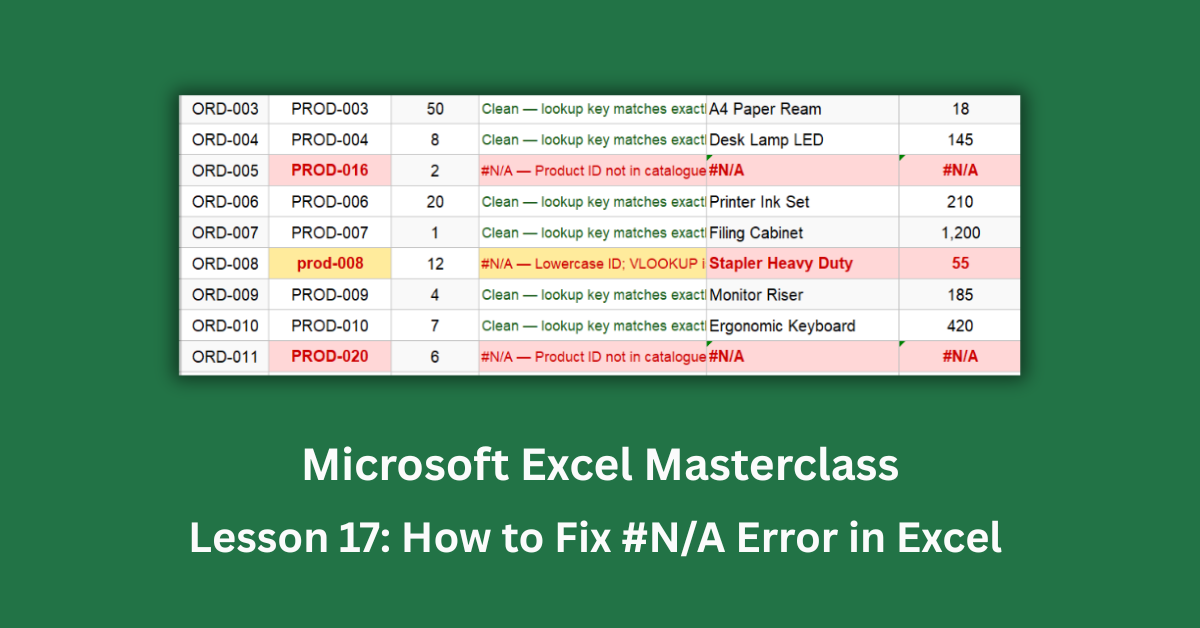
In the order dataset, orders ORD-005, ORD-011, ORD-017, and ORD-023 reference product codes like PROD-016, PROD-020, and PROD-025. None of these appear in the product catalogue. VLOOKUP, MATCH, and INDEX/MATCH all return #N/A for every one of those orders.
Before assuming a formula error, search the table directly. Press Ctrl + F and search for the exact value. If Ctrl + F can’t find it, the value genuinely isn’t there — and the formula is telling you something true about your data.
Cause 2: Hidden Spaces in the Lookup Value
This is the cause that catches even experienced users. The lookup value looks correct on screen. The table entry looks identical. And yet VLOOKUP returns #N/A.
The reason is almost always an invisible space character. “PROD-013 ” (with a trailing space) and “PROD-013” (clean) are different strings as far as Excel is concerned. The product catalogue has the clean version; the order form has the version with a trailing space. They look the same but they’re not.
In the order dataset, ORD-013 has “PROD-013 ” with a trailing space, and ORD-015 has ” PROD-015″ with a leading space. Both cause #N/A across every lookup column for those rows.
How to spot it: Click the problem cell and look at the formula bar. Move your cursor to the very beginning and end of the value. If there’s a space before the first character or after the last one, that’s your culprit.
Fix: Use TRIM() inside the lookup.
Instead of =VLOOKUP(B2,table,2,0), use =VLOOKUP(TRIM(B2),table,2,0). TRIM removes all leading, trailing, and extra internal spaces before the lookup runs. Apply TRIM to the lookup value, not the table — cleaning the table would require touching every cell, while cleaning the lookup value is a one-formula fix.
For bulk cleanup of source data, select the affected column, go to Data → Text to Columns, and click Finish without changing anything. This often forces Excel to re-evaluate the column and strip accidental spaces.
Cause 3: Data Type Mismatch
A number stored as text looks identical to a real number on screen. Both show “1001” in the cell. But when VLOOKUP searches for the number 1001 and the table stores “1001” as text, no match is found and #N/A appears.
You can spot text-formatted numbers by their alignment. Real numbers right-align in cells by default. Text left-aligns. If a column of IDs leans left in some rows and right in others, you have a type mismatch.
Fix A: Convert the lookup value to text to match the table: =VLOOKUP(TEXT(B2,”0″),table,2,0). This works when the table stores IDs as text.
Fix B: Convert the table column to numbers. Select the column, go to Data → Text to Columns, click Finish. This forces numeric conversion. Then use a standard numeric lookup value.
Fix C: Use XLOOKUP, which handles type matching more gracefully in many scenarios: =XLOOKUP(B2,id_col,name_col,”Not Found”).
Cause 4: Unsorted Range With Approximate Match
VLOOKUP’s fourth argument controls the match type. FALSE (or 0) means exact match — this is what most people use. TRUE (or 1) means approximate match, which requires the first column of the lookup table to be sorted in ascending order. If it’s not sorted, VLOOKUP may return a completely wrong value or #N/A.
Most beginners don’t realise there’s a default here. If you omit the fourth argument entirely, VLOOKUP defaults to TRUE — approximate match. This means =VLOOKUP(B2,table,2) without a FALSE at the end will behave differently from =VLOOKUP(B2,table,2,0). For most lookup scenarios, you want 0 (exact match) and should always include it explicitly.
Fix: Always specify the fourth argument as 0 or FALSE: =VLOOKUP(B2,table,2,0). If approximate match is genuinely needed, sort the first column of your table ascending before running the lookup.
How to Fix #N/A Error in Excel
The IFERROR Approach
=IFERROR(VLOOKUP(B2,table,2,0),”Not Found”) wraps the lookup formula and catches any error it produces — not just #N/A, but all error types. If the lookup fails for any reason, “Not Found” appears instead.
For numeric columns like price or quantity, return 0 rather than text: =IFERROR(VLOOKUP(B2,table,4,0),0). This prevents the #N/A from cascading into downstream calculations like totals and line amounts.
I’ve found that adding IFERROR to every lookup in a shared report is good practice regardless of whether errors are currently appearing. Data quality in collaborative spreadsheets is rarely perfect. Having the fallback built in from the start means a new user entering a wrong code doesn’t break the whole report.
The XLOOKUP Alternative
If you’re on Excel 2019 or Microsoft 365, XLOOKUP is the cleaner option. It has a built-in [if_not_found] argument that eliminates the need for a separate IFERROR wrapper:
=XLOOKUP(B2,id_range,name_range,”Not Found”)
The syntax is simpler and the intent is clearer. You’re saying directly: look for B2 in this column, return the corresponding value from this other column, and if you don’t find it, return “Not Found.” No nesting required.
XLOOKUP also searches left as well as right, handles multiple return columns at once, and doesn’t require the lookup column to be the leftmost column in the range. For anyone still using VLOOKUP as their primary lookup function, switching to XLOOKUP for new work is worth the hour it takes to get comfortable with the syntax.
Microsoft’s XLOOKUP documentation includes comparison examples against VLOOKUP and INDEX/MATCH that make the advantages concrete.
Handling Cascading #N/A
When a lookup column returns #N/A, any formula that references that column inherits the error. A line total of =C2*F2 produces #N/A when F2 (price) shows #N/A. The multiplication isn’t the problem — the upstream lookup is.
Fix the upstream formula first. Once the VLOOKUP or MATCH includes IFERROR and returns 0 instead of #N/A, the line total formula resolves automatically. There’s no need to touch it.
If you can’t fix the upstream formula (perhaps someone else owns that column), wrap the downstream formula instead: =IFERROR(C2*F2,0). This is a valid workaround but not the ideal solution — fixing the root cause is always cleaner.
The MATCH Function and INDEX/MATCH
MATCH returns the position of a value within a range. When the value doesn’t exist, it returns #N/A just like VLOOKUP. The same fixes apply: IFERROR wrapping, TRIM for space issues, type checking for number/text mismatches.
For INDEX/MATCH combinations, IFERROR wraps the whole expression: =IFERROR(INDEX(price_col,MATCH(B2,id_col,0)),0). When MATCH can’t find B2, it returns #N/A. INDEX inherits that #N/A. IFERROR catches it before it reaches the cell.
A Simple Diagnostic Routine
When you see #N/A in a lookup column, work through this in order:
Press Ctrl + F and search for the exact value from the lookup cell. If it’s not found, the value isn’t in the table. If it is found, the issue is something subtle — spaces, data type, or match type.
Click the lookup cell. Look for extra spaces in the formula bar. Run =ISNUMBER(B2) and =ISTEXT(B2) to confirm the data type. Check whether the matching cell in the lookup table has the same type.
Once the cause is clear, the fix is one of three things: IFERROR for missing values, TRIM for spaces, or TEXT/VALUE for type conversion.
Open the practice file’s first sheet to see all three error types across the order dataset, then compare with the Fixed sheet to see each formula corrected. The N/A Causes reference tab maps every scenario to its exact fix in one place.