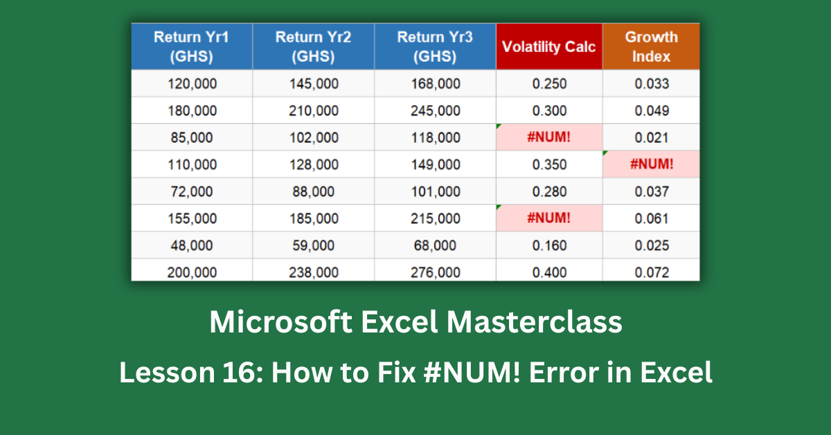
The #NUM! error in Excel means a formula tried to produce a number that doesn’t exist — at least not as a real number Excel can work with. It’s not a data entry mistake like #VALUE!, and it’s not a broken reference like #REF!. It’s a mathematical problem. The formula is asking Excel to calculate something that has no valid numeric answer.
That sounds abstract, but the causes are surprisingly concrete. Taking a square root of a negative number, calculating a logarithm of zero, asking the IRR function to find a rate of return in a cash flow that has no negative investment — these are all mathematically impossible calculations, and #NUM! is Excel’s way of saying so. Understanding why each one is impossible makes the fix obvious.
This post covers every cause of the #NUM! error with step-by-step fixes for each one. Examples come from a financial investment dataset with 20 projects, where five different #NUM! triggers appear across dedicated columns — from negative variance values breaking a SQRT formula to exponents large enough to overflow Excel’s maximum number limit.
Quick Takeaways:
- #NUM! means the calculation has no valid numeric result. The most common trigger is feeding a negative number to SQRT or LOG, which have no real-number solutions for negative inputs.
- Wrap SQRT with ABS() to handle negative numbers: =SQRT(ABS(A2)) always works regardless of sign.
- IRR returns #NUM! when all cash flows are the same sign. At least one value must be negative (the investment) and at least one must be positive (the return).
- POWER and EXP can overflow Excel’s maximum number (~9.99 × 10^307). Cap large exponents with MIN() to prevent this.
- RATE, YIELD, and similar financial functions fail when parameters are financially impossible. Check that payment and present value have opposite signs.
What Causes the #NUM! Error in Excel
Unlike most Excel errors, #NUM! is rooted in mathematics rather than data entry. The formula syntax is correct. The cell references are valid. The numbers simply don’t produce a calculable result given the mathematical rules of the operation.
Cause 1: SQRT or POWER of a Negative Number
The square root of a negative number doesn’t exist in the real number system. =SQRT(-4) has no answer — not a small answer, not an approximate one, literally none. Excel communicates this with #NUM!.
In the investment dataset, seven projects have negative variance values. The formula =SQRT(variance) works correctly for positive variances and breaks immediately when variance goes negative. The formula isn’t wrong — the input is invalid for that operation.
Fix: Use ABS() to force a positive input.
=SQRT(ABS(A2)) takes the absolute value before applying the square root. If a negative variance represents a data entry error, fix the source data instead. But if your workflow occasionally produces negative values, ABS() handles them cleanly.
For cases where the sign matters and a negative input is genuinely invalid, an IF guard is clearer: =IF(A2>=0,SQRT(A2),”Negative input”). This makes the formula’s intent explicit rather than silently converting the value.
Cause 2: LOG or LN of Zero or a Negative Number
Logarithms have two restrictions. LOG(0) equals negative infinity — a value Excel can’t represent. LOG of any negative number has no real solution at all.
In the dataset, column H calculates a growth index using =LOG(growth_base). Three projects have a growth_base of zero or less. Those rows immediately show #NUM!.
Fix: Guard the input with IF.
=IF(A2>0,LOG(A2),”N/A”) checks the value before attempting the logarithm. If the cell might be blank or zero due to missing data (common in early-stage project tracking), IFERROR also works: =IFERROR(LOG(A2),”N/A”).
One approach I’d advise against: substituting a very small positive number like 0.0001 to avoid the error. That technically prevents #NUM! but changes the actual calculation, which can silently corrupt financial analysis. If LOG of a given input is undefined, the formula should say so rather than calculate a meaningless answer.
Microsoft’s function reference for LOG confirms the domain restriction and lists the error conditions.
Cause 3: IRR When Cash Flows Don’t Change Sign
The IRR (Internal Rate of Return) function works by iterating through possible rates until it finds one where the net present value of the cash flow series equals zero. This requires at least one negative and one positive value in the series — without a sign change, there’s no rate that satisfies the equation.
A common mistake: feeding IRR a series of all positive numbers. This happens when someone passes only the returns without the initial investment. =IRR({120000, 145000, 168000}) produces #NUM! because all values are positive — there’s no investment to compare against.
Fix: Ensure the initial investment is negative.
The cash flow series should start with a negative number representing the money going out: =IRR({-500000,120000,145000,168000}). The negative first value is the investment; the positive values are the returns. IRR can now find the rate that balances them.
For situations where the IRR genuinely can’t be found (highly irregular cash flows with multiple sign changes), IFERROR provides a safe fallback: =IFERROR(IRR(range),”No IRR”). The alternative is MIRR (Modified IRR), which uses explicit financing and reinvestment rates instead of solving iteratively, making it more robust for complex cash flow patterns.
Cause 4: POWER or EXP Produces a Number Too Large for Excel
Excel’s maximum representable number is approximately 9.99 × 10^307. =POWER(1.1,999) asks Excel to calculate 1.1 raised to the 999th power — a number roughly 10^41, which would exceed that limit if it weren’t for the overflow. Excel returns #NUM! instead.
In the investment dataset, three projects have compound factor exponents above 500. The formula =POWER(1.1,exponent) produces #NUM! for all three because the result overflows Excel’s numeric ceiling.
Fix: Cap the exponent with MIN().
=POWER(1.1,MIN(A2,300)) ensures the exponent never exceeds 300, keeping the result well within Excel’s limits. The number 1.1^300 is approximately 2.6 × 10^12 — large but representable.
Before applying this fix, ask whether an exponent above 300 is physically meaningful in your context. A compound growth factor of 10^41 isn’t a realistic financial projection — it’s usually a data entry error or an unconstrained formula applied to bad input. Fixing the data is better than capping the formula.
EXP(x) has the same constraint. Values above approximately 709.8 overflow: =EXP(800) produces #NUM!. Guard with =IF(A2<709,EXP(A2),”Overflow”).
Cause 5: RATE, YIELD, or Financial Functions Cannot Converge
Financial functions like RATE, YIELD, XIRR, PRICE, and DURATION use iterative algorithms — they make repeated guesses, checking whether each gets closer to the answer. If the parameters make the financial scenario impossible, the iteration never converges and #NUM! appears.
The most common trigger for RATE: payment and present value having the same sign. =RATE(24, 5000, 100000) gives a positive payment (money coming in) with a positive present value (money coming in) — that’s not a loan, it’s a mathematically incoherent scenario.
Fix: Observe the sign convention.
Outgoing cash is negative. Incoming cash is positive. For a standard loan: you receive money now (positive present value) and make monthly payments (negative). The correct formula is =RATE(24,-C4/24,C4) where the negative sign on the payment reflects money going out.
When parameters might be borderline, wrapping with IFERROR and a meaningful label beats a cryptic error: =IFERROR(RATE(24,-C4/24,C4),”Check signs”).
Two Less Common Causes Worth Knowing
PERCENTILE With k Outside 0 to 1
=PERCENTILE(range,90) looks like it’s asking for the 90th percentile. It’s actually asking for the 90th value — a k value of 90, which is 90 times the valid maximum of 1. The result is #NUM!. The correct formula is =PERCENTILE(range,0.9). Think of k as a decimal, not a percentage.
DATE With an Out-of-Range Year
Excel’s date system runs from January 1, 1900 (serial number 1) to December 31, 9999. Any year outside that range — including year 0, negative years, or year 10000 — produces #NUM!. This usually occurs in dynamic date calculations where a formula subtracts a large number of months and accidentally goes before 1900. Guard with: =IF(AND(year>=1900,year<=9999),DATE(year,month,day),”Out of range”).
The Fastest Diagnostic Process
When you see #NUM!, click the cell and read the formula bar. Identify the function being used. Then ask one question: does the input I’m passing meet the mathematical requirements of that function?
For SQRT and POWER with fractional exponents: is the base positive?
For LOG and LN: is the input greater than zero?
For IRR: does the series contain at least one negative value?
For RATE: do the payment and present value have opposite signs?
For PERCENTILE: is k between 0 and 1 as a decimal?
The general safety net — =IFERROR(formula,”Check input”) — prevents #NUM! from cascading into downstream formulas. But treat IFERROR as a last line of defence, not a first response. Fix the mathematical problem where you can. When the error truly represents an expected edge case (a new project with no returns yet, a log calculation before the data populates), IFERROR with a meaningful label is appropriate and professional.
Open the practice file and compare the error columns in Sheet 1 against the corrected formulas in Sheet 2. The Mathematical Constraints Reference tab maps every function to its valid input range in one place — useful to bookmark for financial modelling work.